This is the second post in 3Blue1Brown’s Compression is Intelligence series. Part 1 rewrote entropy from scratch, so this one picks up right there: after entropy, what on earth is a language model’s loss function, and why that one. Original video: But what is cross-entropy? — Compression is Intelligence Part 2 (also mirrored on Bilibili with Chinese subtitles). After this one, cross-entropy finally clicked for me in a completely different way — I used to just memorize the formula.
1. An Experiment From Twenty Years Ago
The story starts with a 2002 paper, Language Trees and Zipping. What it did is a bit wild: throw texts written in different languages into an off-the-shelf compressor (gzip), look at the resulting file sizes, and you can classify the languages and even recover the family tree among them.
No training, no dictionary, no word-frequency statistics, not even any linguistic prior. Just compression.
That idea is worth sitting with: why can a compressor see language relationships? Because at its core it is estimating the statistical regularities of the data — how far a text can be squeezed depends on how predictable it is. The closer two languages are, the more compressing B with A’s contexts looks like compressing A alone.
In other words, “compression distance” is naturally a measure of difference between distributions. That measure later gets a name: cross-entropy.
To be fair, the video says this itself: compression distance is not strictly cross-entropy, and gzip is nowhere near the Shannon limit — this is only an empirical estimate. But the direction is right, and it is enough to walk us from “compression” to the door of “language model training”.
2. Encoding a Toy Message
Natural language distributions are too complicated to describe, so the video starts with a toy: sending commands to a remote robot, with only four symbols — up, down, left, right.
The first version of the distribution (the old routine):
| Symbol | Probability |
|---|---|
| up | 1/2 |
| down | 1/4 |
| left | 1/8 |
| right | 1/8 |
Part 1 already derived the conclusion: in the optimal code, each symbol gets −log₂(probability) bits.
| Symbol | Probability | Bits |
|---|---|---|
| up | 1/2 | 1 |
| down | 1/4 | 2 |
| left | 1/8 | 3 |
| right | 1/8 | 3 |
The −log₂ shape feels awkward at first. Shannon called it the information content of an event. Grant even jokes that he hopes historians will call it log base 1/2, because it is really asking “how many times do you have to fold something in half to get this many pieces”.
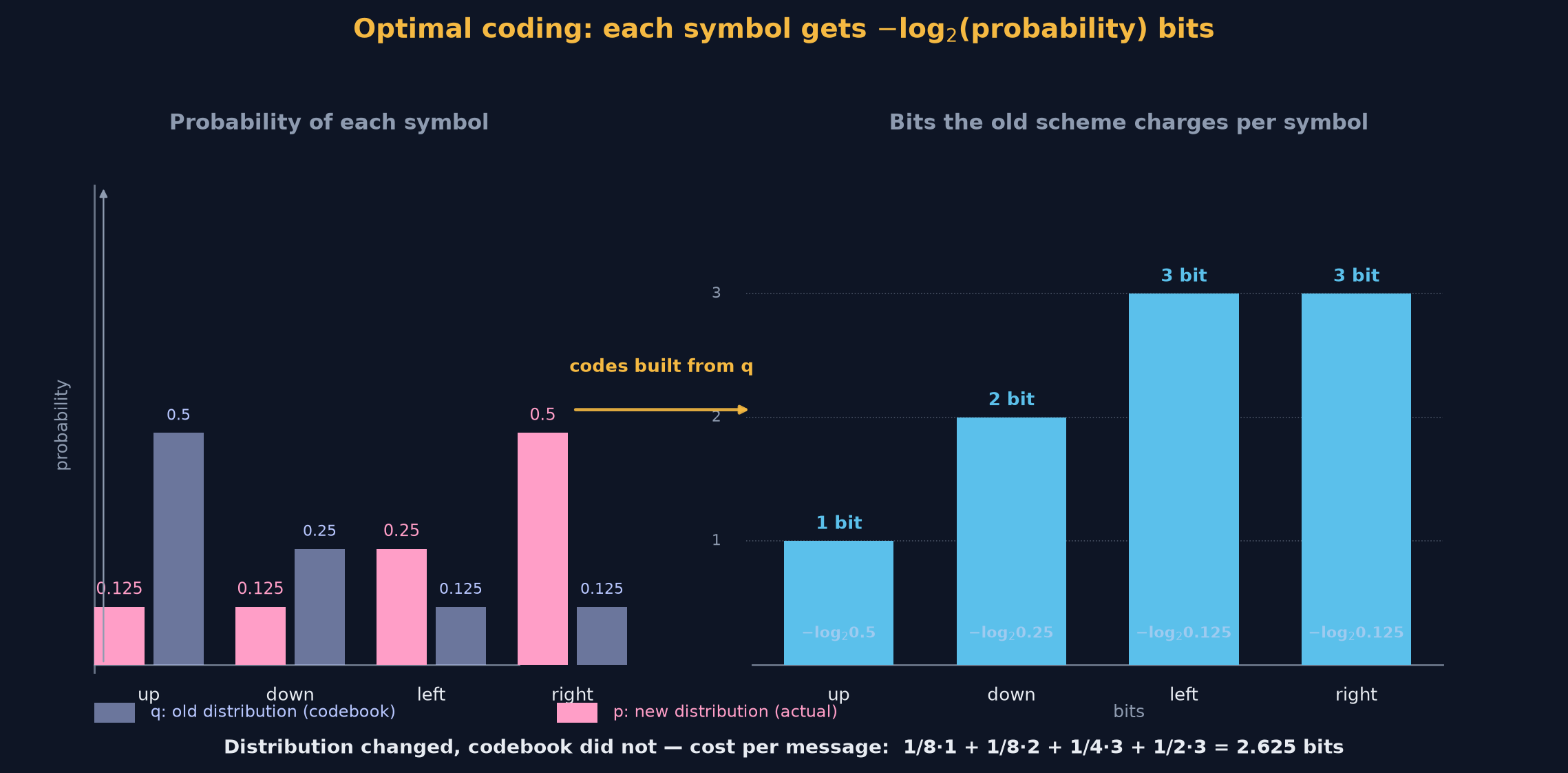
Then the plan changes. From now on, the new distribution is:
| Symbol | Probability |
|---|---|
| up | 1/8 |
| down | 1/8 |
| left | 1/4 |
| right | 1/2 |
Notice this: the encoder and decoder are already frozen, built from the old distribution’s optimal scheme.
So how many bits does each message cost now? A weighted sum:
1/8 · 1 + 1/8 · 2 + 1/4 · 3 + 1/2 · 3 = 2.625 bits per message
2.625 is the cross-entropy of the old distribution with respect to the new one.
It answers a very concrete question: a compression scheme optimized for one context — can you still use it in a different one? Yes, but how much more will it cost?
3. The Cross-Entropy Formula
Generalizing the symbols: call the true distribution p (what actually happens) and the distribution the coding is based on q (what scheme we code with).
H(p || q) = -Σ pᵢ log₂ qᵢ = Σ pᵢ · (-log₂ qᵢ)
Each −log₂ qᵢ term is the “price q charges for symbol i”, multiplied by pᵢ — how often that symbol actually occurs. Sum them up and you get the average bits spent.
In code:
import numpy as np

p = np.array([0.125, 0.125, 0.25, 0.5])   # true distribution (new)
q = np.array([0.5, 0.25, 0.125, 0.125])   # distribution used for coding (old codebook)

cross_entropy = -(p * np.log2(q)).sum()     # 2.625
entropy_p     = -(p * np.log2(p)).sum()     # 1.75
kl            = cross_entropy - entropy_p    # 0.875
Three numbers; everything below uses them.
4. p and q Cannot Be Swapped
Reduce to a two-event distribution and the properties of cross-entropy show up much more clearly.
Case A: q is uniform (50/50), p is skewed (90/10).
0.9 × (-log₂ 0.5) + 0.1 × (-log₂ 0.5) = 0.9·1 + 0.1·1 = 1.00 bits
Case B: flipped — q is skewed (90/10), p is uniform (50/50).
0.5 × (-log₂ 0.9) + 0.5 × (-log₂ 0.1) = 0.5·0.15 + 0.5·3.32 ≈ 1.74 bits
Same two distributions, 90/10 and 50/50, just swapping roles — 1 bit becomes 1.74 bits.
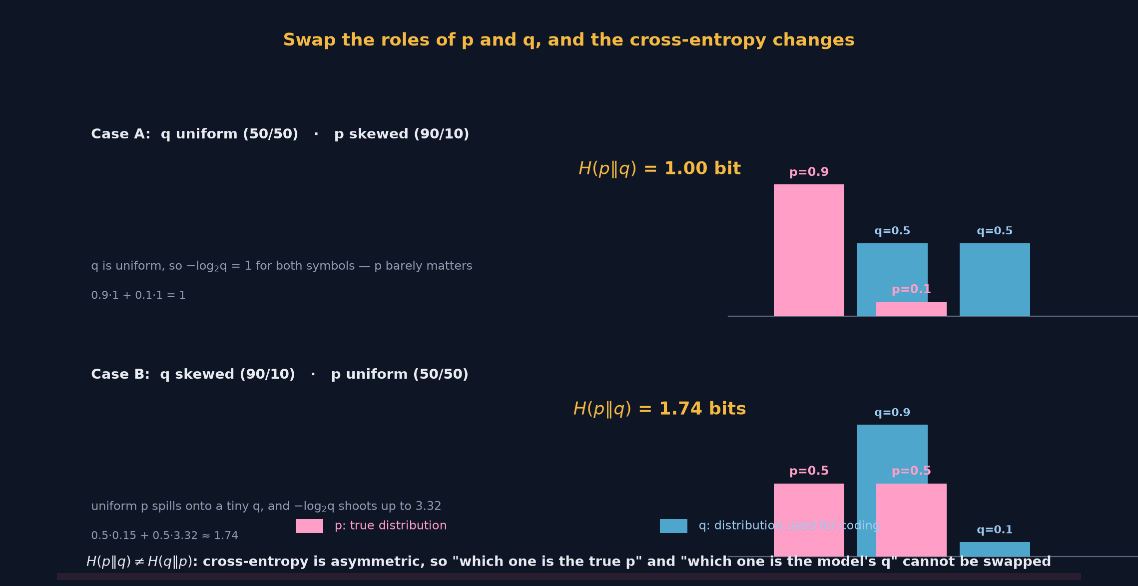
The reason lives in the “unit price” −log₂ q. A skewed q means one symbol is priced at 3.32 bits; when p is also uniform and spills 50% of its mass onto that symbol, 3.32 gets pulled into the average. Flip it around: with a uniform q every symbol costs 1, so no matter what p looks like, the weighted average is still 1.
So H(p||q) ≠ H(q||p). In code, passing the wrong argument in for p produces a bug. In a language model: p is the real data (what the next token actually is) and q is the model’s predictive distribution. Reverse the order and you are not computing the same thing at all.
5. The Floor Is the Entropy
Pin p down and let q move; watch what cross-entropy does.
import numpy as np

p = np.array([0.125, 0.125, 0.25, 0.5])       # fixed true distribution
q_old = np.array([0.5, 0.25, 0.125, 0.125])   # old codebook

ts = np.linspace(0, 1, 200)                   # q slides from p toward q_old
ce = np.array([-(p * np.log2((1-t)*p + t*q_old)).sum() for t in ts])

print(f"q=p:      {ce[0]:.4f}   (= entropy of p)")     # 1.75
print(f"q=old:    {ce[-1]:.4f}")                       # 2.625
print(f"gap (KL): {ce[-1] - ce[0]:.4f}")               # 0.875
q=p:      1.7500   (= entropy of p)
q=old:    2.6250
gap (KL): 0.8750
The curve climbs from the bottom up, and its minimum sits exactly at q = p, where the value is the entropy of p, H(p) = 1.75.
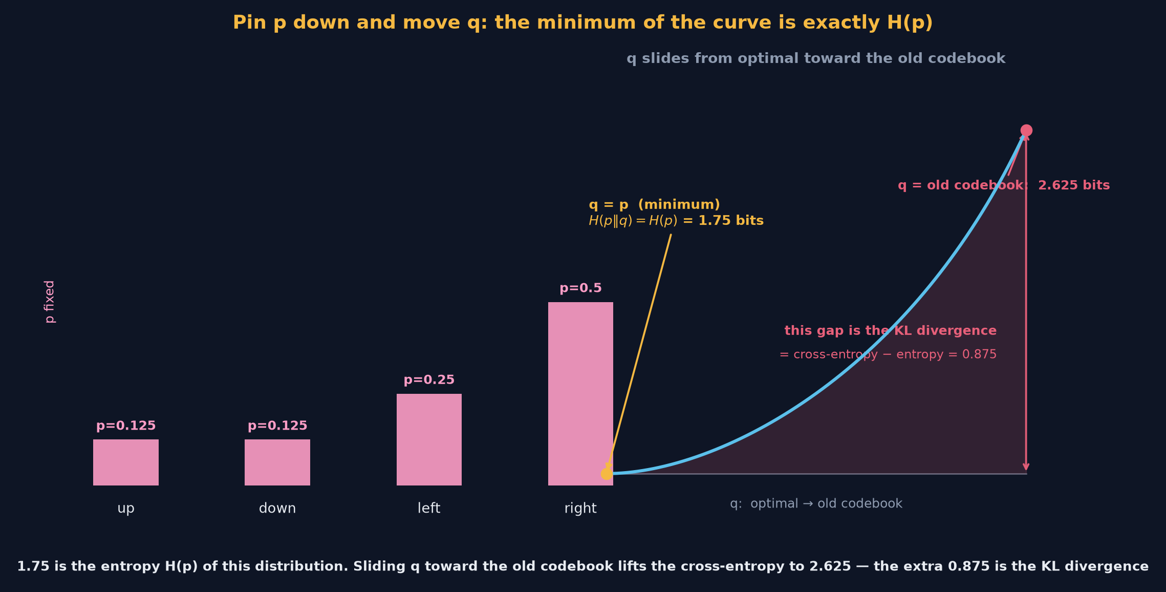
That curve matters: entropy is not just an abstract number — it is a lower bound on the bits any coding scheme can use. Move q away from p a little and cross-entropy lifts a little; how much you lift it by is exactly how much you waste.
That gives KL divergence a definition along the way:
D_KL(p || q) = H(p||q) − H(p)
Cross-entropy minus entropy is “the bits wasted per symbol by using a suboptimal code”. In the example above: 2.625 − 1.75 = 0.875. In machine learning it is often used as a distance between distributions — zero when they agree, larger the further they drift — but it is not symmetric, so it is not a true distance (it fails symmetry).
6. Why the Formula Has to Be −log
Everything before showed what cross-entropy looks like; this section answers why it can only be this.
A language model’s loss is an “average loss”. What property should it have? The most natural one: the average loss is minimized exactly when the model’s distribution q equals the true distribution p, and every other q is worse.
So what loss function F(q) achieves that?
The model produces a distribution q over the possible next tokens, and what we minimize is this weighted average loss:
L(q) = Σ pᵢ F(qᵢ) subject to: Σ qᵢ = 1
An easy detail to miss: L is a function of q, but p is a fixed fact of the real world — differentiate with respect to q only; pᵢ is a constant weight. If you get stuck on that, everything after breaks.
Introduce the Lagrange multiplier λ:
∂L/∂qᵢ = pᵢ F'(qᵢ) + λ = 0
This holds for every i, so:
F'(qᵢ) = -λ / qᵢ (identical in form for all i, i.e. F' is a 1/q)
Integrate:
F(q) = -λ log q + C
Then a boundary condition pins down the constant: when there is only one possible outcome and the prediction is right (q = p = 1), the loss should be 0. Substituting, F(1) = -λ·0 + C = 0, so C = 0.
Thus F(q) = −λ log q; take λ = 1 (merely a choice of units, equivalent to changing the base) and we get:
F(q) = -log q
The average loss is cross-entropy — and it is the only function of this shape.
In other words, cross-entropy was not “chosen”; it was “squeezed out”. Once you accept that “the average loss should be minimized exactly at q = p”, −log is the only answer.
Here is what only hit me when I read to this point: in the earlier sections cross-entropy grew naturally out of the compression path (information content, bits, coding). In this section it is squeezed out of a completely different place on the machine learning path, via constrained optimization. Two entirely unrelated chains of reasoning land on the same formula.
7. The Loss Function of Large Language Models
Now put it all together.
What a large language model does is simple: chop the text into tokens, feed them in, have the model output a probability distribution q over the next token, then compare it with the real next token (that is p). The loss is the negative log of the score the model gives the true token, averaged over all tokens:
L = - (1/N) Σ log q(true token)
Written as cross-entropy, this is “the cross-entropy of the model’s distribution q with respect to the true distribution p”. Section 6 proved this loss is minimized exactly when the model has learned the statistics of the data (q close to p).
A few details:
- Code almost always uses
lograther thanlog₂. That is one constant factor,1/ln 2, which the learning rate absorbs, while the natural log differentiates far more cleanly. - The endgame of pretraining is to drive the loss toward the entropy of language. That entropy is the lower bound (the bottom of the curve in section 5); you never reach it, but you can keep approaching it.
- Mathematically it is extremely clean, engineering-wise extremely complex: batching, optimizers, numerical stability (softmax followed by log produces NaN easily — use
logsumexpinstead). None of that is about the math, but none of it can be avoided either.
8. Compression Is Intelligence
Back to the title. Rephrase the “average information content from the model’s viewpoint” of section 7:
The model’s loss is how many bits it thinks each token is worth. Add up those “model-viewpoint bits” over the whole text, and you have just done one pass of compression.
So training a language model is mathematically equivalent to training an optimal text compressor. This is not an analogy; it is two readings of one and the same objective function.
Here is how I now read the claim: it holds strictly in mathematics — cross-entropy is simultaneously the expected bits of compression and the loss of prediction, with proof paths that do not overlap yet corroborate each other. But “intelligence” is still half a teaching device: compressing well does not mean understanding. What Grant is really doing is putting both sides under one formula and letting you decide how deep to press on that equals sign.
Knowledge distillation is another direct application: have a small model approximate the full distribution the large model produces at the same position, with the loss being the cross-entropy of the small model’s distribution with respect to the large model’s. The win is that every sample receives supervision from an entire distribution instead of a single one-hot label — one training sample then carries far more information than the label alone.
9. References and Reproduction
- Original video: But what is cross-entropy? — Compression is Intelligence Part 2 (mirrored on Bilibili with Chinese subtitles)
- First in the series: Reinventing Entropy — Compression is Intelligence Part 1
- Series playlist: Compression is Intelligence
- Opening experiment: Language Trees and Zipping (Joshi et al., 2002)
Every number in the text can be reproduced from the two code blocks in sections 3 and 5, plain numpy:
- Cross-entropy 2.625 bits per message (old codebook vs new distribution)
H(p) = 1.75bits (entropy of the new distribution, the lower bound on cross-entropy)D_KL = 0.875bits (cross-entropy − entropy)- Asymmetry check:
H(p=90/10, q=50/50) = 1.00vsH(p=50/50, q=90/10) ≈ 1.74
If this write-up was useful to you, I’d love to hear from you.
-
Previous
千卡训练的隐形账单:通信不是瓶颈The Hidden Bill of Thousand-GPU Training: Communication Is Not the Bottleneck -
Next
交叉熵:语言模型的损失函数,为什么只能是它Cross-Entropy: The Loss Function of Language Models, and Why It Must Be This One
If this post helped you, a coffee is always welcome ☕