Yesterday, in MLSys·im Roofline Tutorial Notes, I learned to judge whether a workload is compute-bound or memory-bound in five lines of code, using arithmetic intensity and the ridge point. Today I moved on to the second stage of the Datawhale mlsysim study activity, covering The Memory Wall and Two Phases, One Request. This pushes yesterday’s “static” roofline toward two questions that matter in production: how much faster does a hardware upgrade actually get you, and how does the bottleneck shift as an LLM request generates tokens?
1. The Memory Wall: the Binding Constraint Decides the Speedup
Yesterday’s roofline told us a workload hits whichever ceiling comes first. Today’s question goes one step further — when you upgrade to a faster GPU, which spec does the speedup actually track?
The tutorial gives a punchy table:
| Regime | Binding constraint | Speedup |
|---|---|---|
| Memory-Bound | HBM bandwidth (TB/s) | Bandwidth ratio between GPUs |
| Compute-Bound | Peak FLOP/s | FLOP/s ratio between GPUs |
Now look at the A100 → H100 specs:
| Spec | A100 | H100 | Ratio |
|---|---|---|---|
| Peak FP16 | 312 TFLOP/s | 989 TFLOP/s | 3.2x |
| HBM bandwidth | 2.04 TB/s | 3.35 TB/s | 1.7x |
| Ridge point (FLOP/byte) | 153.0 | 295.2 | — |
Compute grew 3.2x, bandwidth only 1.7x. It is easy to conclude: if your workload is memory-bound, the speedup ceiling when moving to an H100 is 1.7x — the extra 1.5x of compute is entirely wasted.
Verify with Llama-3-8B at batch size 1 (FP16 weights = 8B params × 2 bytes = 16 GB):
| A100 | H100 | Speedup | |
|---|---|---|---|
| Bottleneck | Memory | Memory | — |
| Latency | 9.00 ms | 5.60 ms | 1.6x |
| Throughput | 111.1 tok/s | 178.5 tok/s | — |
Sanity check: 16 GB / 2.04 TB/s ≈ 8.0 ms, and 16 GB / 3.35 TB/s ≈ 4.8 ms — the engine’s reported latency is essentially “the time to stream the weights once from HBM,” and it matches the bandwidth ratio. This is the memory wall: the GPU’s compute is starving for data, and you paid 3.2x for compute that never gets used.
The trend is more worrying. The tutorial lines up three generations:
| GPU | TFLOP/s | BW (TB/s) | Ridge | 8B bs=1 latency | Bottleneck |
|---|---|---|---|---|---|
| V100 | 125.0 | 0.90 | 138.9 | 19.97 ms | Memory |
| A100 | 312.0 | 2.04 | 153.0 | 9.00 ms | Memory |
| H100 | 989.0 | 3.35 | 295.2 | 5.60 ms | Memory |
Compute doubles every generation while bandwidth grows only half as fast, pushing the ridge point ever higher — meaning more and more production workloads land on the memory-bound side of the new hardware. The memory wall is not a thing of the past; it gets thicker every year.
2. My Reproduction: a Fully Memory-Bound Batch Sweep and the “Plateau”
The task (E1+E2) asks for a batch-size sweep to find the ridge-point crossover on the A100 and H100. I swept batch size from 1 all the way to 8192:
| Batch | A100 Bottleneck | H100 Bottleneck | Speedup | A100 Throughput (tok/s) | H100 Throughput (tok/s) |
|---|---|---|---|---|---|
| 1 | Memory | Memory | 1.6x | 111.1 | 178.5 |
| 4 | Memory | Memory | 1.6x | 352.1 | 568.0 |
| 16 | Memory | Memory | 1.6x | 768.7 | 1,250.5 |
| 64 | Memory | Memory | 1.6x | 1,091.8 | 1,787.4 |
| 256 | Memory | Memory | 1.6x | 1,219.9 | 2,002.3 |
| 1024 | Memory | Memory | 1.6x | 1,256.8 | 2,064.4 |
| 4096 | Memory | Memory | 1.6x | 1,266.4 | 2,080.5 |
| 8192 | Memory | Memory | 1.6x | 1,268.0 | 2,083.2 |
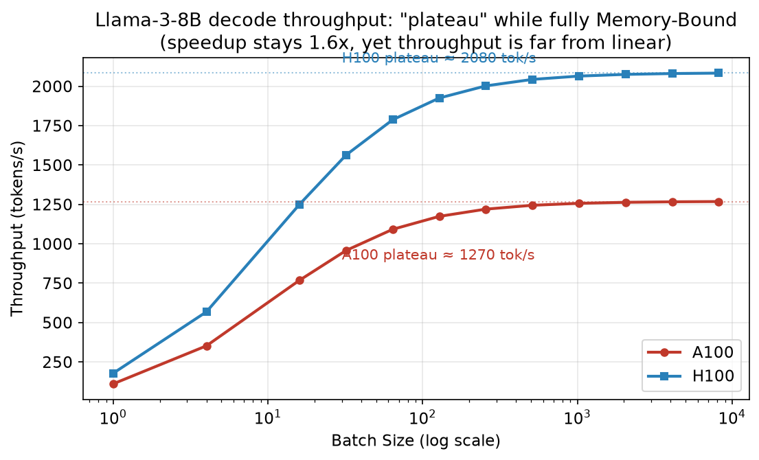
Figure 1: Memory-Bound all the way to batch 8192, speedup pinned at 1.6x (= bandwidth ratio). Throughput plateaus after batch ≈ 256 — far from linear.
Three findings:
- No crossover anywhere. This contrasts sharply with yesterday’s ResNet-50, which flipped to Compute at batch=2. The reason: LLM decoding is autoregressive — every token must stream the entire weight set from HBM, so the arithmetic intensity is pinned at the 1 FLOP/byte scale (8B model: 2P FLOPs and 2P bytes per token), two orders of magnitude below the A100’s 153 and the H100’s 295. The decode ridge-point crossover does not exist in any practical batch range — to feed the compute by growing the batch, you would run out of memory first.
- Speedup is pinned at 1.6x. Both GPUs are memory-bound the whole way; the contest is the bandwidth ratio, 3.35/2.04 ≈ 1.64. This is Section 1’s conclusion, live on the bench.
- Throughput does not grow linearly; it plateaus. From batch 1 to 8192, throughput only went 111 → 1268 (~11x) while the batch grew 8192x. This raised my first question of the day — detailed in Section 5, Q1.
3. Two Phases, One Request: Two Walls Inside a Single Request
The Memory Wall answers “does upgrading help?”; Two Phases answers “why does the same model on the same GPU bottleneck on completely different resources for the first token vs. the 100th token?”
LLM generation is autoregressive, so one request naturally splits into two phases:
- Prefill: the entire prompt (say 2048 tokens) goes through one parallel forward pass to produce the first token. All input tokens compute simultaneously, saturating the GPU’s compute units — it hits the compute wall. Its latency is TTFT (Time To First Token).
- Decode: every subsequent token runs a full forward pass but processes only one new token, while streaming the entire weight set (8B params = 16 GB) from HBM — it hits the memory wall. Its latency is ITL (Inter-Token Latency).
The tutorial’s key line: prefill’s arithmetic intensity is ~2048 FLOP/byte (2048 tokens in parallel, weights reused 2048 times), far above the H100’s ridge of 295; decode’s is ~1 FLOP/byte, far below. The same weights, loaded the same way, two completely different operating regimes.
The previous Engine.solve models inference as a single forward pass and returns one latency number. For the two-phase case you use ServingModel, which models each phase separately and outputs TTFT and ITL:
from mlsysim.solvers import ServingModel
solver = ServingModel()
r = solver.solve(model=model, hardware=hardware, seq_len=2048, batch_size=1, precision="fp16")
# TTFT prefill: 70.97 ms   ITL per token: 5.19 ms
Two numbers, two stories. More importantly, the two metrics respond asymmetrically to hardware upgrades. The tutorial runs 8B across three GPU generations:
| GPU | TFLOP/s | BW (TB/s) | TTFT (ms) | ITL (ms) |
|---|---|---|---|---|
| A100 | 312 | 2.04 | 225.0 | 8.33 |
| H100 | 989 | 3.35 | 70.97 | 5.19 |
| H200 | 989 | 4.80 | 70.97 | 3.72 |
- A100 → H100: compute 3.2x → TTFT improves ~3x; bandwidth 1.7x → ITL improves ~1.7x.
- H100 → H200: compute unchanged → TTFT unchanged; bandwidth 1.4x → ITL improves 1.4x.
I reproduced this on the H100 with the 70B model (O3: how model scale amplifies the two phases); the pattern holds exactly:
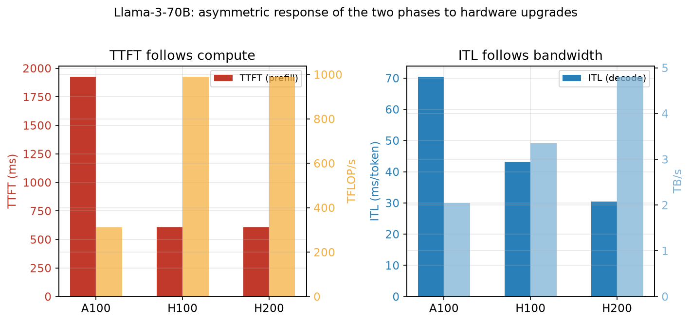
Figure 2: Llama-3-70B on A100/H100/H200 — TTFT strictly follows compute (989 unchanged → 607 ms unchanged), ITL strictly follows bandwidth (3.35 → 4.80 TB/s → 43.15 → 30.36 ms).
| GPU | TFLOP/s | BW (TB/s) | TTFT (ms) | ITL (ms) |
|---|---|---|---|---|
| A100 | 312 | 2.04 | 1,924.2 | 70.38 |
| H100 | 989 | 3.35 | 607.0 | 43.15 |
| H200 | 989 | 4.80 | 607.0 | 30.36 |
70B magnifies both walls: FP16 weights are 141.2 GB, TTFT jumps to the second scale (600 ms floor), and ITL grows ~8x (5.19 for 8B → 43.15 for 70B). Also note that the engine reports a Memory utilization of 165.2% — 70B FP16 does not fit on a single H100 (80 GB). That is the memory wall’s other form: the capacity wall, which I come back to in Section 6.
The decoupling rule — TTFT only tracks compute, ITL only tracks bandwidth — is the foundation of all LLM serving cost analysis.
4. Quantization: It Saves Decode, Not Prefill
Since decode streams all weights from HBM every token, wouldn’t shrinking the weights directly speed it up? That is the logic of quantization. The tutorial verifies it with 8B (O2):
| Precision | TTFT (ms) | ITL (ms) | Weights |
|---|---|---|---|
| fp16 | 70.97 | 5.19 | 16.06 GB |
| int8 | 35.47 | 2.76 | 8.03 GB |
| int4 | 70.97 | 1.54 | 4.02 GB |
My 70B reproduction (weights 141.2 → 70.6 → 35.3 GB):
| Precision | TTFT (ms) | ITL (ms) | Weights |
|---|---|---|---|
| fp16 | 607.0 | 43.15 | 141.2 GB |
| int8 | 303.4 | 21.97 | 70.60 GB |
| int4 | 607.0 | 11.39 | 35.30 GB |
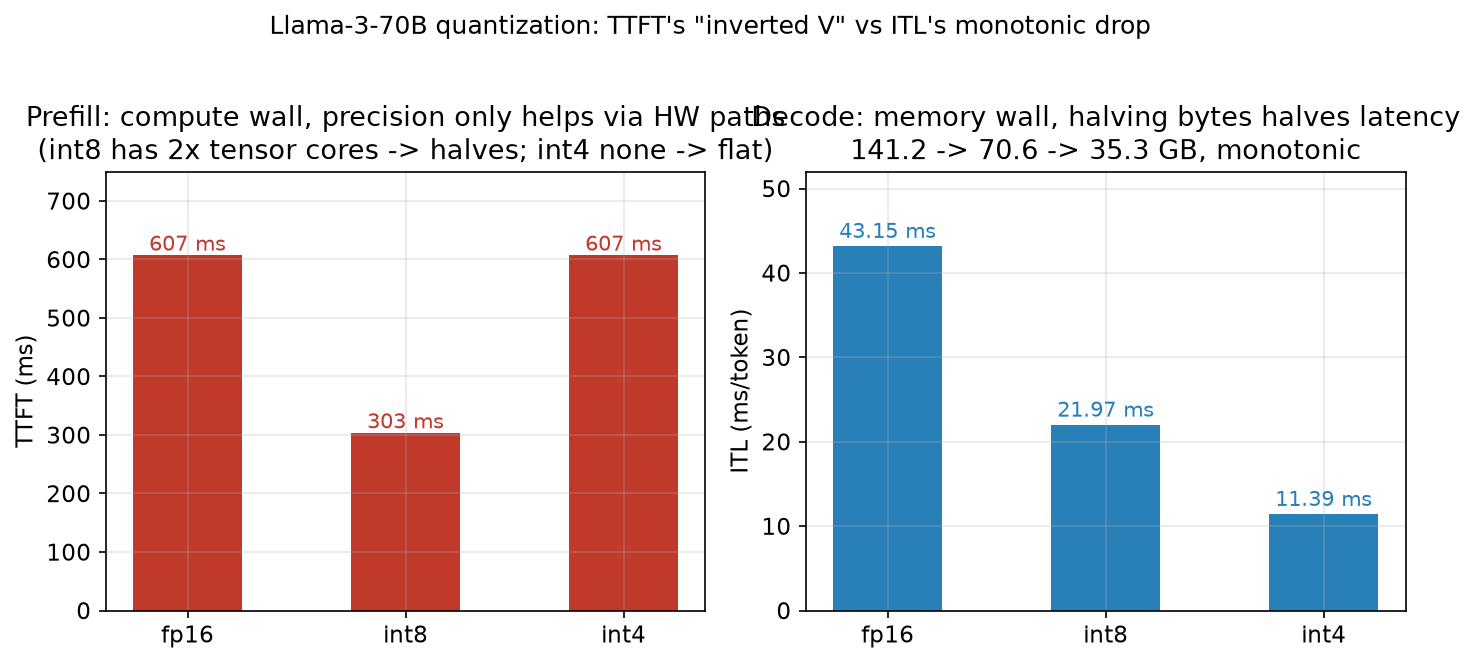
Figure 3: ITL drops monotonically with byte count (memory wall: halve the bytes, halve the latency); TTFT shows an “inverted V” — halves at int8, bounces back at int4.
Two crisp patterns:
- Decode side: halve the weight bytes, halve the ITL. 5.19 → 2.76 → 1.54; 43.15 → 21.97 → 11.39. Decode is “stream all weights per token,” so byte count is the whole game.
- Prefill side: a counter-intuitive “inverted V.” At int8, TTFT halves (70.97 → 35.47, 607 → 303.4) — quantization seems to help prefill too; but at int4, TTFT “bounces back” to the fp16 level. That looks like it violates the intuition that smaller weights should be faster, yet it turned out to be the most technically interesting question of the day (my fifth question; root cause in Section 5, Q5).
One-sentence summary: quantization mainly saves decode; prefill sits on the compute wall, and smaller weights don’t compute faster unless the hardware actually has a matching low-precision compute path.
5. Questions from My Learning Process
Q1: If everything is Memory-Bound, why doesn’t throughput grow linearly — why does the growth keep slowing down?
This was the first thing I noticed in the batch sweep. Intuition: with fixed bytes per sample and a fixed memory ceiling, throughput should scale linearly with batch; saturation should only appear after crossing into the compute-bound regime.
The answer has three stages: at small batch, fixed overhead (dispatch tax + per-layer framework tax) dominates, pinning throughput low; as batch grows, that fixed overhead gets amortized, and throughput enjoys a stretch of near-linear growth; at large batch, before compute ever gets fed, HBM bandwidth is already exhausted by streaming all weights (plus the linearly growing KV cache), so throughput enters a plateau. The measurements confirm it: on the A100, batch 1→16 grows throughput ~7x, 16→64 only 1.4x, and 1024→8192 is essentially flat (1256 → 1268). “Memory-Bound” does not imply “linear throughput” — fixed overhead and the plateau are two different things. That distinction was one of the biggest takeaways of the day.
Q2: Isn’t batch size a hardware property? Why does the assignment ask “what are the ridge points of the A100 and the H100, and why do they differ?”
The ridge point = peak FLOP/s ÷ peak bandwidth is a hardware constant, independent of batch: A100 ≈ 153 FLOP/byte, H100 ≈ 295 FLOP/byte. They differ because the two generations pair different compute/bandwidth ratios (the H100 got 3.2x compute with only 1.7x bandwidth, pushing its ridge up).
What does batch affect, then? The workload’s arithmetic intensity: weights are read from HBM once but reused by every sample in the batch, so a bigger batch means FLOPs grow linearly while bytes barely move. Arithmetic intensity rises, the operating point slides right along the roofline slope, until it crosses the ridge into the compute-bound region. The ridge is the hardware’s terrain; arithmetic intensity is the workload’s position — and batch size is the knob that moves the position. The confusion in the question comes from mistaking a workload property for a hardware property.
Q3: The tutorial says TTFT is tens of milliseconds (dominated by the 989 TFLOP/s compute ceiling) and ITL is a fraction of a millisecond (dominated by the 3.35 TB/s bandwidth ceiling) — where do those numbers come from?
Hand-compute it for Llama-3-8B (32 layers, hidden 4096, seq_len 2048, H100, efficiency 0.5):
- Prefill linear layers: 2 × params × tokens = 2 × 8.03B × 2048 ≈ 32.9 TFLOP; attention (QK^T and AV): ~2.2 TFLOP; total ≈ 35 TFLOP.
- TTFT = 35 TFLOP ÷ (989 TFLOP/s × 0.5) ≈ 70.97 ms — identical to the engine’s output, digit for digit.
- ITL = 16.06 GB ÷ 3.35 TB/s ≈ 4.8 ms (the full weight stream; plus the 0.268 GB KV cache and per-layer framework tax → ≈ 5.19 ms).
The cleanest verification is a “perturbation experiment”: double compute, keep bandwidth → TTFT halves, ITL unchanged; double bandwidth, keep compute → ITL halves, TTFT unchanged. Whichever metric a perturbation moves tells you which ceiling dominates it — two rows of contrast and the dual-wall story is settled.
Q4: For decode, why “2P FLOPs and 2P bytes per token”? Don’t the weights have only P parameters?
This is a units trap: P is the parameter count; 2P bytes is the FP16 footprint — each parameter takes 2 bytes. 8B params = 16 GB = 2P bytes. So per token: FLOPs = 2P (one multiply-accumulate per weight, 1 MAC = 1 FLOP convention), bytes = 2P, and arithmetic intensity = 2P ÷ 2P = 1 FLOP/byte. The KV cache is an extra load, but at 0.27 GB it’s negligible next to the 16 GB of weights. My earlier confusion mixed up “parameter count” with “byte count.”
Q5: Why does fp16 → int8 halve TTFT, but int4 bounces it back up? Shouldn’t weight precision be irrelevant to a compute wall?
The most counter-intuitive question of the day. The root cause is in the engine source. ServingModel picks the prefill compute rate like this:
peak_flops_prefill = hardware.compute.precision_flops.get(precision, hardware.compute.peak_flops)
i.e. look up the hardware’s low-precision compute table by precision; fall back to the FP16 peak if the entry is missing. Here is the H100 table:
H100: {'tf32': 494, 'fp8': 1979, 'int8': 1979}   # no int4 entry!
B200: {'fp8': 4500, 'int4': 9000}                # int4 only appears on B200
- int8: the table has 1979 TFLOP/s (= 2 × 989), so TTFT halves — the engine faithfully models the H100’s INT8 tensor-core acceleration path.
- int4: not in the table → falls back to 989, TTFT returns to the fp16 level — the hardware fact is that the H100 has no native dense INT4 compute; INT4 usually has to be packed into INT8 to run. The B200 is the first card with an official INT4 rate (9000 TFLOP/s).
So the “inverted V” is not an engine bug; it is the simulator being faithful to its hardware table, and the hardware table being faithful to real silicon. Quantization pays off instantly on the decode side (bytes are the whole game), but on the prefill side it only helps if the hardware has a matching low-precision compute path — which is exactly why “int4 weights + fp16 compute” mixed-precision schemes dominate production.
Q6: Exercise 2 (chatbot vs. summarizer) needs input and output token counts, but ServingModel only takes seq_len — how do you run it?
ServingModel.solve accepts a single seq_len parameter; there is no separate input/output argument. After going in circles, I worked it out myself: total generation time = TTFT (prefill of all input) + N × ITL (one decode step per output token), so just take the two numbers and multiply — chatbot (50 input / 500 output) ≈ TTFT + 500 × ITL; summarizer (4000 input / 100 output) ≈ TTFT + 100 × ITL. This also settles Exercise 2’s conclusion by hand: the chatbot is ITL-dominated (buy bandwidth), the summarizer is TTFT-dominated (buy compute).
6. Three Details from Reading the Engine Source
Continuing yesterday’s habit, I peeled open the ServingModel formulas and the hardware tables:
Detail 1: the complete two-phase formulas.
# Prefill: linear layers 2P·S + attention 4·L·H·head_dim·S², divided by
# "precision-scaled compute × efficiency", plus dispatch tax
prefill_ops = (2·P·S + 4·L·H·head_dim·S²) · batch
t_prefill = prefill_ops / (peak_flops_prefill × efficiency) + dispatch_tax

# Decode: stream "weights + KV cache" once per token, plus per-layer framework tax
t_decode_per_token = (weights_bytes + kv_cache_bytes) / bandwidth + layers × 10μs
Two things worth noting: first, prefill explicitly contains the O(S²) attention term — at long context, attention compute overtakes the linear layers, which foreshadows the “KV-Cache hidden tax” tutorial and long-context scenarios; second, decode also pays the layer tax per token (32 layers × 10 μs ≈ 0.32 ms), so fixed overhead exists on decode too — which is why small models at small batch have slightly higher ITL than the pure bandwidth estimate.
Detail 2: prefill compute is looked up by precision — precision_flops.get(precision, peak_flops). This is the root cause of Q5, and the most vivid lesson that “the simulator’s default parameters and hardware tables are part of the model”: without reading the source, you can’t know what assumptions the engine made on behalf of the hardware.
Detail 3: the memory wall has two forms — a bandwidth wall and a capacity wall. 70B FP16 inference reports 165.2% memory utilization; it doesn’t fit on one H100. The capacity wall decides “how big a model / how many concurrent users one card can serve,” while the bandwidth wall decides “how fast each token is.” Yesterday was all about the bandwidth wall; today I found that the capacity wall constrains deployment shape just as hard (tensor parallelism, quantization, KV-cache limits).
7. Personal Takeaways
-
The memory wall thickens every generation — ask about the regime before buying hardware. The ridge point across three generations rose from 138.9 to 295.2, so the same workload is more likely to land memory-bound on newer hardware. “Buy a faster card” on a memory-bound workload means paying at the bandwidth ratio — answer “which side of the roof is my production workload on” before choosing the card.
-
“One request, two walls” is the foundation of serving cost analysis. The latency budget of one LLM request is TTFT + N × ITL, each part hitting its own wall. A chatbot (short prompt, long reply) is ITL-dominated → buy bandwidth. A summarizer (long document, short output) is TTFT-dominated → buy compute. Same model, different business shape, possibly opposite procurement strategies.
-
Quantization saves decode, not prefill — which explains why mixed precision is everywhere. int4 weights cut decode’s streaming cost to a quarter, while fp16 compute keeps prefill accurate and fast. Two phases, two precisions: that is the engineering landing of this asymmetry.
-
The simulator’s hardware table is part of the model. TTFT bouncing back at int4 is not a bug; it’s a faithful projection of the fact that the H100 has no native INT4 compute path. Before making decisions with a simulator, find out what assumptions its defaults and spec tables made for you — the biggest shared takeaway from two days of reading source code.
-
A first-order analysis can draw decision boundaries before you spend a dollar. The SLA selection experiments (tutorial’s 8B run: T4/A100 eliminated at TTFT < 200 ms, H100/H200 pass; my 70B run with TTFT < 500 ms fails everything) show the value is not precise prediction, but ruling out the cards you shouldn’t even consider.
8. Next Steps & References
- Tutorial chain: 00 Hello Roofline (Part 1) → 01 The Memory Wall (this post) → 02 Two Phases, One Request (this post) → KV-Cache: The Hidden Tax (concurrency limits) → Quantization: Not a Free Lunch → The $9M Question.
- Task: Datawhale llm-algo-leetcode #83
- Reproduce:
pip install mlsysim; scripts in the appendix below. - Environment: WSL2 + conda env mlsysim (python 3.11, mlsysim 0.1.1), no GPU required.
Appendix: Complete Runnable Scripts
Script 1: Memory Wall experiment (E1+E2) — Llama-3-8B batch sweep on A100/H100, hunting the ridge-point crossover
import mlsysim
from mlsysim import Engine
from mlsysim.show import table

a100 = mlsysim.Hardware.Cloud.A100
h100 = mlsysim.Hardware.Cloud.H100

flops_a = a100.compute.peak_flops.to("TFLOPs/s").magnitude
flops_h = h100.compute.peak_flops.to("TFLOPs/s").magnitude
bw_a = a100.memory.bandwidth.to("TB/s").magnitude
bw_h = h100.memory.bandwidth.to("TB/s").magnitude

print(f"A100: {flops_a} TFLOP/s, {bw_a} TB/s, ridge = {flops_a/bw_a:.1f} FLOP/byte")
print(f"H100: {flops_h} TFLOP/s, {bw_h} TB/s, ridge = {flops_h/bw_h:.1f} FLOP/byte")

model = mlsysim.Models.Language.Llama3_8B

# Single point: batch=1, verify "3.2x compute buys only 1.6x speedup"
pa = Engine.solve(model=model, hardware=a100, batch_size=1, precision="fp16")
ph = Engine.solve(model=model, hardware=h100, batch_size=1, precision="fp16")
print(f"A100: {pa.bottleneck}, {pa.latency.to('ms')}, {pa.throughput}")
print(f"H100: {ph.bottleneck}, {ph.latency.to('ms')}, {ph.throughput}")
print(f"Speedup = {pa.latency.to('ms').magnitude / ph.latency.to('ms').magnitude:.1f}x")

# Batch sweep: find the crossover (conclusion: LLM decode is memory-bound all the way)
rows = []
for batch in [1, 4, 16, 32, 64, 128, 256, 512, 1024, 2048, 4096, 8192]:
    pa = Engine.solve(model=model, hardware=a100, batch_size=batch, precision="fp16")
    ph = Engine.solve(model=model, hardware=h100, batch_size=batch, precision="fp16")
    la = pa.latency.to("ms").magnitude
    lh = ph.latency.to("ms").magnitude
    sp = la / lh if lh > 0 else 0
    rows.append([batch, pa.bottleneck, ph.bottleneck, f"{sp:.1f}x", pa.throughput, ph.throughput])

table(["Batch", "A100 Bottleneck", "H100 Bottleneck", "Speedup", "A100 Throughput", "H100 Throughput"], rows)
Script 2: Two-phase experiment (E3+E4+O2+O3+O4) — ServingModel TTFT/ITL analysis, quantization comparison, and SLA-based selection
import mlsysim
from mlsysim.solvers import ServingModel
from mlsysim.show import table, info

# Llama-3-70B (swap to mlsysim.Models.Language.Llama3_8B for 8B)
model = mlsysim.Models.Language.Llama3_70B
hardware = mlsysim.Hardware.Cloud.H100

solver = ServingModel()
result = solver.solve(
    model=model,
    hardware=hardware,
    seq_len=2048,       # 2K token context window
    batch_size=1,       # single user
    precision="fp16"
)

info("Phase Analysis",
     TTFT_prefill=result.ttft.to('ms'),
     ITL_per_token=result.itl.to('ms'))

info("Memory Budget",
     Model_weights=result.model_weights_size,
     KV_cache=result.kv_cache_size,
     Memory_utilization=f"{result.memory_utilization:.1%}")

# E4: across generations — TTFT only tracks compute, ITL only tracks bandwidth
gpus = [
    ("A100", mlsysim.Hardware.Cloud.A100),
    ("H100", mlsysim.Hardware.Cloud.H100),
    ("H200", mlsysim.Hardware.Cloud.H200),
]
rows = []
for name, hw in gpus:
    r = solver.solve(model=model, hardware=hw, seq_len=2048, batch_size=1, precision="fp16")
    rows.append([name, hw.compute.peak_flops.to("TFLOPs/s"),
                 hw.memory.bandwidth.to("TB/s"), r.ttft.to('ms'), r.itl.to('ms')])
table(["GPU", "TFLOP/s", "BW (TB/s)", "TTFT (ms)", "ITL (ms)"], rows)

# O2: quantization — ITL drops monotonically (bytes halve), TTFT only responds to HW low-precision paths
rows = []
for prec in ["fp16", "int8", "int4"]:
    r = solver.solve(model=model, hardware=hardware, seq_len=2048, batch_size=1, precision=prec)
    rows.append([prec, r.ttft.to('ms'), r.itl.to('ms'), r.model_weights_size])
table(["Precision", "TTFT (ms)", "ITL (ms)", "Weights"], rows)

# O4: SLA-based selection — with TTFT<500ms and ITL<50ms, which GPUs qualify (70B: all FAIL)
gpus_all = [
    ("T4",   mlsysim.Hardware.Cloud.T4),
    ("A100", mlsysim.Hardware.Cloud.A100),
    ("H100", mlsysim.Hardware.Cloud.H100),
    ("H200", mlsysim.Hardware.Cloud.H200),
]
TTFT_SLA, ITL_SLA = 500, 50  # ms
rows = []
for name, hw in gpus_all:
    r = solver.solve(model=model, hardware=hw, seq_len=4096, batch_size=1, precision="fp16")
    ttft = r.ttft.to("ms").magnitude
    itl = r.itl.to("ms").magnitude
    rows.append([name, f"{ttft:.1f} ms", f"{itl:.2f} ms",
                 "✓" if ttft <= TTFT_SLA else "✗",
                 "✓" if itl <= ITL_SLA else "✗",
                 "PASS" if ttft <= TTFT_SLA and itl <= ITL_SLA else "FAIL"])
table(["GPU", "TTFT", "ITL", "TTFT OK?", "ITL OK?", "Verdict"], rows)
If this note helps you, feel free to reach out.
-
Previous
用 5 行代码预测模型瓶颈:MLSys·im Roofline 教程学习笔记Predicting Model Bottlenecks in 5 Lines of Code: MLSys·im Roofline Tutorial Notes -
Next
内存墙与两阶段:为什么 3.2 倍算力只换来 1.6 倍加速The Memory Wall & Two Phases: Why 3.2x More FLOPS Buys Only 1.6x Speedup
If this post helped you, a coffee is always welcome ☕