Recently I joined Datawhale’s mlsysim study activity, and the assignment format pushed me to systematically learn the mlsysim simulation framework from MLSysBook. Over the past two days I worked through the introductory tutorial Hello, Roofline, going from “picking a GPU by VRAM size alone” to “predicting a performance bottleneck in five lines of code” — quite a haul. This post is both a study summary and a collection of the conceptual pitfalls I hit and the small details I dug up by reading the engine source.
1. The Roofline Model: Performance Bottlenecks in Four Lines of Math
The roofline model comes from Williams et al.’s classic 2009 paper and is the bedrock of ML systems performance analysis. Its core idea is extremely plain: every accelerator has two ceilings, and you always hit whichever one comes first:
- Compute ceiling: how many floating-point operations the chip can do per second, in FLOP/s. The A100’s FP16 peak is 312 TFLOP/s.
- Memory bandwidth ceiling: how much data can be moved from HBM per second, in byte/s. The A100’s HBM2e bandwidth is 2.04 TB/s.
The decision procedure is just three lines:
T_compute = FLOPs / peak compute
T_memory  = Bytes / peak bandwidth
T = max(T_compute, T_memory)   → the larger term decides the bottleneck
Two key concepts:
- Arithmetic Intensity (AI) = FLOPs ÷ Bytes: how many floating-point operations you get per byte moved. High AI means the workload is compute-dense; low AI means it is data-dense.
- Ridge Point = peak compute ÷ peak bandwidth: where the workload’s AI sits relative to the ridge point directly decides the bottleneck type.
The rule is simple: AI < ridge point → Memory-Bound (the GPU goes hungry waiting for data — adding compute won’t help); AI > ridge point → Compute-Bound (bandwidth feeds it fine; the bottleneck is compute itself).
A handy analogy: picture the GPU as a chef and HBM bandwidth as the kitchen pass. Arithmetic intensity is “how many cuts you get per trip to the pantry.” One cut per food run → memory-bound; dozens of cuts per run → compute-bound.
⚠️ Two easy pitfalls (the tutorial calls them out explicitly):
- FLOP counting convention: industry convention counts 1 multiply-accumulate (MAC) = 2 FLOPs, while the MLSys Zoo counts 1 MAC = 1 FLOP. This makes every number differ by 2x — the A100’s ridge point is ~312 FLOP/byte under the 2-FLOP convention but ~156 under the 1-FLOP convention. Before comparing any number from any paper or any tool, first confirm which convention it uses.
- The roofline is an upper bound, not a prediction: real performance, because of scheduling overhead, memory-access patterns, and imperfect utilization, usually reaches only 40%–60% of the roof. Its value is not precise latency reporting — it is telling you which resource is constraining you.
2. Getting Started with MLSys·im: Running End to End in 5 Steps
The value of mlsysim: no real GPU, no framework install, not one line of CUDA — an “model × hardware” performance prediction on your laptop within 30 seconds. The core API boils down to two calls:
import mlsysim
from mlsysim import Engine

# 1. Pull "audited" model and hardware specs straight from the Zoo — no datasheet digging
model = mlsysim.Models.Vision.ResNet50        # 25.6M params, 4.1 GFLOP per inference
hardware = mlsysim.Hardware.Cloud.A100        # 312 TFLOP/s, 2.04 TB/s

# 2. One-line solve: model + hardware + config → bottleneck, latency, throughput
profile = Engine.solve(model=model, hardware=hardware, batch_size=1, precision="fp16")
print(profile.bottleneck, profile.latency, profile.throughput)
# → Memory  0.543 ms  1843 images/s

# 3. Sweep batch size to watch the bottleneck flip; plot_roofline for one-click visualization
None of this needs real hardware — and that is exactly its teaching value: build intuition with a first-order model first, then verify on real machines.
3. Experiments and Results
3.1 ResNet-50 × A100: Batch Sweep and the Bottleneck Flip
Setup: ResNet-50 (25.6M params = 51.2 MB in FP16, 4.1 GFLOP per inference), A100, FP16. Engine.solve defaults to a compute efficiency of efficiency=0.5, so the effective ridge point = 312 × 0.5 ÷ 2.039 ≈ 76.5 FLOP/byte (the theoretical ridge point is 312 ÷ 2.039 ≈ 153).
| Batch | Latency (ms) | Throughput (img/s) | Bottleneck |
|---|---|---|---|
| 1 | 0.543 | 1,843 | Memory |
| 2 | 0.568 | 3,524 | Compute |
| 4 | 0.620 | 6,450 | Compute |
| 8 | 0.725 | 11,031 | Compute |
| 16 | 0.936 | 17,103 | Compute |
| 32 | 1.356 | 23,598 | Compute |
| 64 | 2.197 | 29,130 | Compute |
| 128 | 3.879 | 32,997 | Compute |
| 256 | 7.243 | 35,343 | Compute |
Key findings:
- The crossover sits at batch=2: AI jumps from 72.8 at batch=1 to 133.5 at batch=2, clearing the effective ridge of 76.5 in one step. The reason is intuitive — when you grow the batch, FLOPs double strictly, but the model weights are loaded from HBM only once, so bytes barely move and AI naturally explodes.
- Throughput grows 19.2x, but marginal gains decay fast: batch 1→2 gives +91%, 2→4 gives +83%, 32→64 only +23%, 128→256 just +7%. Once past the ridge, the bottleneck switches to compute and throughput gradually approaches the hardware’s compute ceiling.
- The MFU view: at batch=1 the Model FLOPs Utilization on this A100 is only 2.4%, and only at batch=256 does it reach 46.4% (the engine ships an
mfufield). That is the quantified evidence behind the tutorial’s line “most of the A100’s 312 TFLOP/s is idle.”
3.2 A100 vs H100: A Faster Card Doesn’t Automatically Pay Off
H100 specs: 3.2x the A100’s compute (989 TFLOP/s), but only 1.64x the bandwidth (3.35 TB/s). Compute and bandwidth grew asymmetrically, pushing the ridge point higher: effective ridge = 989 × 0.5 ÷ 3.35 ≈ 147.6.
The comparison:
| Batch | A100 Bottleneck | H100 Bottleneck | H100 Throughput (img/s) |
|---|---|---|---|
| 1 | Memory | Memory | 1,898 |
| 2 | Compute | Memory | 3,785 |
| 4 | Compute | Compute | 7,364 |
| 32 | Compute | Compute | 41,273 |
| 128 | Compute | Compute | 81,463 |
Two very counter-intuitive conclusions:
- At batch=1, the H100 is only 3% faster than the A100 (1,898 vs 1,843 img/s). Both are memory-bound, so the contest is bandwidth: 3.35 vs 2.04 TB/s ≈ 1.64x, but scattered latency overheads dilute the gap. Paying several times more for the card buys no corresponding speedup.
- The H100’s crossover comes later (batch=4 vs batch=2). The higher the ridge, the bigger the batch needed to “feed” the compute. Only at batch=128 does the H100 pull out a 2.47x lead — by then both are deeply compute-bound.
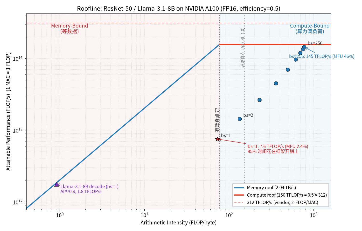
Figure 1: arithmetic intensity of each workload versus the hardware ridge point. The blue region is compute-bound, the red region memory-bound. Note that the actual working point of batch=1 ResNet-50 (7.6 TFLOP/s) sits far below the memory roof (148 TFLOP/s) — direct evidence that fixed overheads exist; expanded below.
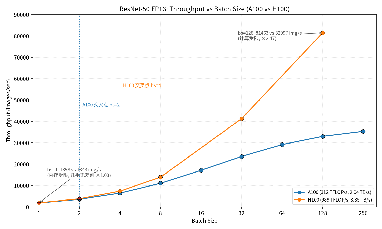
Figure 2: throughput versus batch size on both GPUs. Nearly coincident at small batch (both memory-bound); the gap opens to 2.5x at large batch.
3.3 Llama-3.1-8B: the Classic “Memory Wall” Workload
Finally, swap the model for Llama-3.1-8B (8.03B params = 16.06 GB, 16.06 GFLOP per token), A100, batch=1:
- Arithmetic intensity AI ≈ 0.91 FLOP/byte (weight reuse rate ≈ 1: for every 2-byte weight read, only about 2 floating-point operations are done), far below any hardware’s ridge point.
- Latency 9.0 ms, throughput 111 tok/s, Memory-Bound.
- The breakdown: T_memory = 8.66 ms vs T_compute = 0.10 ms — the bandwidth bottleneck dominates overwhelmingly.
LLM decoding is autoregressive: it generates one token at a time, yet the entire model weights (plus the KV cache) must pass through HBM. An AI on the order of 1 means it was born standing at the very bottom of the roof’s steepest slope. That is why the optimization direction for LLM inference is never “pile on compute” but reducing data movement: quantization (GPTQ/AWQ), KV cache optimization, operator fusion, PagedAttention…
4. Questions from My Learning Process
While studying I fired a stream of questions at the AI tutor; here are the representative ones, kept exactly where I genuinely got stuck the first time:
Q1: What is HBM in the tutorial? Does “memory bottleneck” mean the computer’s RAM?
HBM (High Bandwidth Memory) is the GPU’s video memory — just not ordinary GDDR: it is high-speed DRAM built with 3D stacking and through-silicon vias (TSV). The A100 uses HBM2e (2.04 TB/s), the H100 HBM3 (3.35 TB/s). The “Memory” ceiling in the roofline is set by HBM bandwidth, nothing to do with the CPU-side system RAM — data movement in GPU inference basically never touches system memory. My early reading of “memory-bound” as “the computer doesn’t have enough RAM” was pointed in a completely wrong direction.
Q2: Is 1 MAC = 1 FLOP or 2 FLOPs? Why does one convention deserve its own paragraph?
Because it makes every conclusion differ by 2x. NVIDIA officially counts one multiply-accumulate as 2 FLOPs, hence the A100’s 312 TFLOP/s badge; the MLSys Zoo counts 1 FLOP, and ResNet-50’s 4.1 GFLOP is on that convention. Mix the two while computing a ridge point and you get 156 and 312 — numbers a full factor apart. Align conventions first, compare numbers second — this line cannot be overstated in performance analysis.
Q3: The tutorial says the two ceilings are “nearly balanced” at batch=1, and also that “most of the compute is idle” — isn’t that contradictory?
No, but it does take a turn. At batch=1, AI ≈ 72.8 (or the tutorial’s rounded 82), which is close in order of magnitude to the ridge point of 156 — close enough to say, loosely, “balanced”; but 72.8 < 156, so it is still on the memory-bound slope and the compute genuinely idles. Measured MFU is only 2.4%. That is what “nearly balanced but memory-bound” means: being close to the passing line is not the same as passing. There are only two ways to put the idle compute to work: grow the batch (push AI over the ridge), or cut the data movement.
Q4: Why does changing batch from 1 to 2 immediately flip the bottleneck from Memory to Compute?
Go back to the definition of AI: the numerator FLOPs doubles linearly with batch, while the denominator Bytes barely moves (weights are loaded once; activations are only a small fraction of the weights). So AI jumps straight from 72.8 to 133.5, clearing the effective ridge of 76.5 in one bound. Batch size is the most direct knob for dialing arithmetic intensity — the biggest hands-on takeaway of this experiment.
Q5: The tutorial’s hand-computed latency is 0.026 ms — why does Engine.solve report 0.543 ms?
This is the question I only fully understood after reading the engine source — see the next section. It is also, I think, my most technically interesting discovery.
5. Two Details Found by Reading the Engine Source
Detail 1: the engine’s latency formula = max(compute, memory) + fixed overhead
Open mlsysim/core/engine.py; the single-node inference latency formula is:
latency = max(T_compute, T_memory) + dispatch_tax + num_layers × 10μs (per-layer tax)
ResNet-50 has 50 layers: a 10 μs per-layer framework tax plus a 0.02 ms dispatch overhead, so the fixed part alone comes to 0.515 ms — while at batch=1 the pure compute/memory time is only 0.026/0.028 ms. In other words, 95% of the latency is “framework tax.” This perfectly explains the tutorial’s low-key line that the latency reported by Engine.solve may differ slightly from hand calculation:
- the hand-computed 0.026 ms is the pure upper bound (an ideal pipeline);
- the engine’s 0.543 ms is the engineering reality of “upper bound + per-layer software overhead.”
It also makes the roofline’s “upper bound” nature very concrete: at small batch, fixed overhead pins the actual performance far below the roof — that huge gap between the batch=1 point and the memory roof in Figure 1 is exactly it. In a real system, when kernels are too small and launched too often, framework overhead takes over the show — which is precisely the foreshadowing for the later tutorials “Two Phases, One Request” and the framework-overhead wall (Wall 7).
Detail 2: the engine defaults to efficiency=0.5, so read the ridge point at half price
Engine.solve has an unassuming default parameter efficiency: float = 0.5; effective compute = peak × efficiency. Which means:
- the decision line on the tutorial’s paper is 156 FLOP/byte (peak under the 1-FLOP convention: 312 ÷ 2.0 TB/s);
- the effective ridge point the engine actually decides against is 76.5 FLOP/byte (312 × 0.5 ÷ 2.039).
So the tutorial says “the batch=1 label depends on the exact assumptions”, while the engine just outputs “Memory” — because the engine’s default assumption (efficiency=0.5) pulled the ridge point down by half. When you use a simulation tool, its default parameters are part of the model too — without reading the source, you have no idea which assumptions it made on your behalf.
6. Personal Takeaways
-
Judge the regime first, then talk optimization. The first thing the roofline taught me: when facing an unfamiliar model, compute AI = FLOPs ÷ Bytes, compare it against the hardware’s ridge point, and only then choose the optimization direction. Memory-Bound → quantize, fuse, cut data movement; Compute-Bound → then pile on compute and tune precision. Get the direction wrong, and no amount of fine-grained optimization is anything but effort on the wrong side of the problem.
-
Batch size is the best value-for-money knob — but it has a ceiling. Doubling the batch at small batch nearly doubles throughput; once past the ridge, the gains decay fast (+91% → +7%). Online serving also has a latency constraint (the bigger the batch, the higher the per-request latency, 0.54 → 7.24 ms), so real deployment means finding the balance point between throughput and latency.
-
“Upgrade the hardware” is not a simple proposition. The H100 has 3.2x the A100’s compute but is only 3% faster on a memory-bound workload. Before choosing a card, answer one question: which side of the roof is my workload on? A fun counterexample while we’re at it: edge devices (e.g. Jetson AGX Orin) have low compute and low bandwidth, yet their compute-to-bandwidth ratio — and hence ridge point — is the highest of all, meaning small models on edge hardware most easily fall into “no matter how you feed it, the compute stays hungry.”
-
LLM inference is a slave of the memory wall. AI ≈ 1 FLOP/byte means: unless you change the essence of the data movement (quantization, caching, sparsification), piling on compute does almost nothing for single-stream latency. That also explains why the inference-framework arms race is about the KV cache and quantization, not the number of SMs.
-
First-order analysis tools deserve heavy use. Simulators like mlsysim max out both “mechanistic explanatory power” and “computation speed” — they don’t chase precision; they chase getting the right intuition in place before you touch anything. While reading the source I also found it ships a complete training-side model (3D parallelism, communication overhead, pipeline bubbles) to dig into next.
7. Next Steps & References
- Tutorial chain: Hello, Roofline (this post) → 01 The Memory Wall (why 3.2x compute doesn’t buy 3.2x speedup) → 02 Two Phases, One Request (prefill compute-bound vs decode memory-bound). Both are written up in English in Part 2 of this series.
- Check-in task: Datawhale llm-algo-leetcode #76
- To reproduce:
pip install mlsysim, then:
import mlsysim
from mlsysim import Engine
model = mlsysim.Models.Vision.ResNet50
hardware = mlsysim.Hardware.Cloud.A100
for bs in [1, 2, 4, 8, 16, 32, 64, 128, 256]:
    p = Engine.solve(model=model, hardware=hardware, batch_size=bs, precision="fp16")
    print(bs, p.bottleneck, f"{p.throughput:.0f}/s")
- Environment: WSL2 + conda env mlsysim (python 3.11, mlsysim 0.1.1), no GPU throughout.
Appendix: Complete Runnable Script (copy and run as-is)
"""
MLSys·im Task 1: Roofline in practice - ResNet50 on A100
Check-in task requirements: https://github.com/datawhalechina/llm-algo-leetcode/issues/76
Tutorial reference: https://mlsysbook.ai/mlsysim/tutorials/00_hello_roofline.html
"""

import mlsysim
from mlsysim import Engine

print(f"✅ mlsysim version: {mlsysim.__version__}")

# ================= 1. Setup: choose model and hardware =================
# Call the built-in model and hardware strictly per the tutorial API
model = mlsysim.Models.Vision.ResNet50
hardware = mlsysim.Hardware.Cloud.A100

print(f"\n📦 Model: {model.name}")
print(f"   - Parameters: {model.parameters:,}")
print(f"   - Inference FLOPs (single image): {model.inference_flops:,}")

print(f"\n🖥️  Hardware: {hardware.name}")
print(f"   - Peak Compute (FP16): {hardware.compute.peak_flops.to('TFLOPs/s')}")
print(f"   - Memory Bandwidth: {hardware.memory.bandwidth.to('TB/s')}")

# ================= 2. Minimal experiment: Single Image Inference =================
print("\n" + "="*60)
print("🔍 Single Image Inference (batch_size=1)")
print("="*60)

profile = Engine.solve(
    model=model,
    hardware=hardware,
    batch_size=1,
    precision="fp16"
)

print(f"   - Latency: {profile.latency.to('ms')}")
print(f"   - Throughput: {profile.throughput}")
print(f"   - Bottleneck: {profile.bottleneck}")

# ================= 3. Batch size sweep =================
print("\n" + "="*60)
print("📊 Batch Size Sweep (1 → 256)")
print("="*60)
print(f"{'Batch':<8} {'Latency(ms)':<14} {'Throughput':<18} {'Bottleneck'}")
print("-" * 60)

batch_sizes = [1, 2, 4, 8, 16, 32, 64, 128, 256]
results = []

for bs in batch_sizes:
    p = Engine.solve(model=model, hardware=hardware, batch_size=bs, precision="fp16")
    results.append(p)
    print(f"{bs:<8} {p.latency.to('ms'):<14} {str(p.throughput):<18} {p.bottleneck}")

# ================= 4. Exercise 2: A100 vs H100 comparison =================
print("\n" + "="*60)
print("✏️  Exercise 2: A100 vs H100 Crossover Comparison")
print("="*60)

h100 = mlsysim.Hardware.Cloud.H100
print(f"H100 Peak Compute (FP16): {h100.compute.peak_flops.to('TFLOPs/s')}")
print(f"H100 Memory Bandwidth: {h100.memory.bandwidth.to('TB/s')}")

print(f"\n{'Batch':<8} {'A100 BN':<15} {'H100 BN'}")
print("-" * 40)

for bs in [1, 8, 32, 64, 128]:
    pa = Engine.solve(model=model, hardware=hardware, batch_size=bs, precision="fp16")
    ph = Engine.solve(model=model, hardware=h100, batch_size=bs, precision="fp16")
    print(f"{bs:<8} {pa.bottleneck:<15} {ph.bottleneck}")

# ================= 5. Exercise 3: Llama-3 8B analysis =================
print("\n" + "="*60)
print("✏️  Exercise 3: Llama-3-8B Memory-Bound Analysis")
print("="*60)

llama = mlsysim.Models.Language.Llama3_8B
p_llama = Engine.solve(model=llama, hardware=hardware, batch_size=1, precision="fp16")

print(f"Model: {llama.name}")
print(f"   - Parameters: {llama.parameters:,}")
print(f"   - Batch=1 Latency: {p_llama.latency.to('ms')}")
print(f"   - Bottleneck: {p_llama.bottleneck}")
print(f"\n💡 Why Memory-Bound?")
print(f"   LLM autoregressive decoding processes ONE token at a time.")
print(f"   FLOPs are tiny (only attention + FFN for 1 token),")
print(f"   but must load ENTIRE KV-Cache + weights from HBM.")
print(f"   → Very low arithmetic intensity → Memory-Bound")
If this note helps you, feel free to reach out.
-
Previous
用 5 行代码预测模型瓶颈:MLSys·im Roofline 教程学习笔记Predicting Model Bottlenecks in 5 Lines of Code: MLSys·im Roofline Tutorial Notes -
Next
内存墙与两阶段:为什么 3.2 倍算力只换来 1.6 倍加速The Memory Wall & Two Phases: Why 3.2x More FLOPS Buys Only 1.6x Speedup
If this post helped you, a coffee is always welcome ☕