In The Memory Wall & Two Phases, I split a single LLM request into two walls: Prefill hits the compute wall, Decode hits the memory wall. Today I moved on to the third stage of the Datawhale mlsysim study activity, flipping the lens from “time” to “space”: where does the memory actually go, and what do you do when the model gets bigger? Corresponding tutorials: KV-Cache: The Hidden Memory Consumer and Quantization: Not a Free Lunch. The core tools switch from
EnginetoServingModel,calc_kv_cache_sizeandCompressionModel— three tools for three questions: how much memory does one request eat, how many requests fit on one card, and what does shrinking the weights actually accelerate?
1. KV-Cache: Where the Memory Goes
Task 2 left us a cliffhanger: a 70B model in FP16 weighs 141.2 GB, far beyond one H100’s 85.9 GB (80 GiB). The “where does memory go” question starts with the weight ledger (E1):
| Model | FP16 | INT8 | INT4 |
|---|---|---|---|
| Llama-3-8B | 16.06 GB | 8.03 GB | 4.02 GB |
| Llama-3-70B | 141.2 GB | 70.6 GB | 35.3 GB |
8B params × 2 bytes = 16.06 GB; 70B × 2 = 141.2 GB. 70B in FP16 doesn’t fit a single card; INT8 (70.6 GB) is marginal and INT4 (35.3 GB) is comfortable — that’s conclusion one, but the bigger question is behind it: even once the weights are in, how much does one 2K-request’s KV-Cache eat?
The KV-Cache is the memory block that caches the K/V matrices of all previous tokens so Decode can reuse them instead of recomputing attention. Its formula:
KV-Cache = 2 × L × n_kv_heads × head_dim × seq_len × batch_size × bytes_per_elem
Every term maps to a Llama-3-8B hyperparameter:
| Symbol | Meaning | Llama-3-8B value |
|---|---|---|
| L | number of layers | 32 |
| n_kv_heads | KV heads (≪ Q heads under GQA) | 8 |
| head_dim | dimension per head | 128 |
| seq_len | sequence length | variable |
| batch_size | concurrent requests | variable |
| bytes_per_elem | bytes per element | FP16=2, INT8=1, INT4=0.5 |
Sanity check for a single request at 2K context:
2 × 32 × 8 × 128 × 2048 × 1 × 2 = 268,435,456 bytes = 0.268 GB
This matches ServingModel.solve()’s kv_cache_size output exactly: 0.268 GB. Hand-calculated, engine-reported, and the official blog all agree. Stretch the sequence length and the E2 ledger looks like this:
| Seq length | KV-Cache per request (8B) | Multiple of 4K |
|---|---|---|
| 2K (2048) | 268 MB | 0.5× |
| 4K (4096) | 537 MB | 1× (baseline) |
| 32K (32768) | 4,295 MB | 8× |
| 128K (131072) | 17,180 MB | 32× |
KV-Cache is strictly linear in sequence length: double the length, double the cache. seq_len is a plain multiplicative factor with no amortization. A single 128K request’s KV-Cache (17.18 GB) already exceeds the model weights (16.06 GB) — long context is not free; it is priced per token.
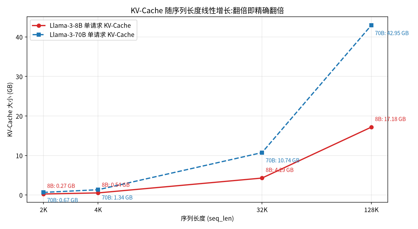
Fig 1: KV-Cache grows linearly with sequence length; both 8B and 70B are exact straight lines (70B has 2.5× the layers, hence the steeper slope).
2. The Capacity Wall: Sequence Length Sets the Concurrency Ceiling
With 16.06 GB of weights inside the 85.9 GB H100, the remaining budget buys KV-Cache. So E3’s core question: given a sequence length, how many requests can one card serve concurrently?
The plain arithmetic: max concurrency = (85.9 − 16.06) ÷ KV-Cache per request. At 4K: 69.84 ÷ 0.537 ≈ 130. Then sweep with ServingModel.solve()’s feasible flag; ground truth for all four lengths:
| Seq length | KV-Cache per request | Max concurrent (feasible) | Pattern |
|---|---|---|---|
| 2K | 268 MB | 260 | baseline |
| 4K | 537 MB | 130 | halved |
| 32K | 4,295 MB | 16 | keeps halving |
| 128K | 17,180 MB | 4 | single digits |
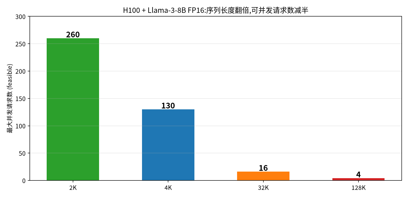
Fig 2: doubling sequence length halves the concurrency ceiling — the direct consequence of KV-Cache’s pure linearity.
The 130 matches the hand calculation, which also confirms that ServingModel’s memory budget is a plain sum of “weights + KV-Cache + system overhead”. Note that at 128K the ceiling is down to 4 — even though a single 128K request is feasible (33.24 GB total), the concurrent capacity is already near zero. Compared to 260 concurrent requests at 2K, 128K context is a cliff in cost-effectiveness.
This is the “capacity wall” — the second form of the memory wall (flagged in Part 2). The bandwidth wall decides how fast each token is; the capacity wall decides how big a model, and how much concurrency, one card can serve. Sequence length is the knob pressing down on the concurrency ceiling.
3. What If the Model Gets Bigger: 8B → 70B and Quantization
O1: Scaling the model scales both phases
Switching from 8B to 70B (FP16, H100, seq 2048, bs 1), measured:
| Metric | Llama-3-8B | Llama-3-70B | Growth |
|---|---|---|---|
| Weights | 16.06 GB | 141.2 GB | 8.8× |
| TTFT (Prefill) | 70.97 ms | 607.0 ms | 8.6× |
| ITL (Decode) | 5.19 ms | 43.15 ms | 8.3× |
Parameters grow 8.8× and both TTFT and ITL follow at ~8× — both phases are linearly dominated by model scale. TTFT because prefill FLOPs scale with parameter count; ITL because decode moves the entire weight matrix per token, so 8.8× the weights means 8.8× the moving time. This confirms the Task 2 conclusion: the bottleneck region doesn’t change as the model grows; both walls just get taller.
E4+E5: Quantization helps Decode, not Prefill
Quantization halves/quarters the weight bytes, with completely asymmetric effects on the two phases (8B, H100, seq 2048):
| Precision | Weights | ITL (Decode) | TTFT (Prefill) |
|---|---|---|---|
| fp16 | 16.06 GB | 5.19 ms | 70.97 ms |
| int8 | 8.03 GB | 2.76 ms (1.9×) | 35.47 ms (2.0×) |
| int4 | 4.02 GB | 1.54 ms (3.4×) | 70.97 ms (1.0×) |
- Decode side: halve the bytes, halve the ITL. 5.19 → 2.76 → 1.54, strictly tracking weight size. Decode moves the whole weight matrix per token; bytes are the lever.
- Prefill side: it only accelerates if the hardware has a low-precision compute path. int8 looks up 1979 TFLOP/s in H100’s precision_flops table and halves TTFT; int4 finds no native INT4 path on H100, falls back to the FP16 peak, and TTFT snaps back — the “inverted V” I traced to the source in Part 2.
One line: quantization rescues Decode, not Prefill.
4. Compression vs Pruning: Saving Storage ≠ Saving Time
Optional experiment O3 uses CompressionModel to compare the two compression routes. I ran both end-to-end (8B, H100):
| Method | Compressed size | Ratio | Accuracy Δ | Speedup | Memory savings |
|---|---|---|---|---|---|
| FP16 (baseline) | 16.06 GB | 2.0× | +0.00% | 2.00× | 50.0% |
| INT8 quantization | 8.03 GB | 4.0× | -0.00% | 4.00× | 75.0% |
| INT4 quantization | 4.02 GB | 8.0× | -0.03% | 8.00× | 87.5% |
| Prune 50% (unstructured) | 16.06 GB | 2.0× | -0.00% | 1.00× | 50.0% |
| Prune 75% (unstructured) | 8.03 GB | 4.0× | -0.04% | 1.00× | 75.0% |
| Prune 90% (unstructured) | 3.21 GB | 10.0× | -0.06% | 1.00× | 90.0% |
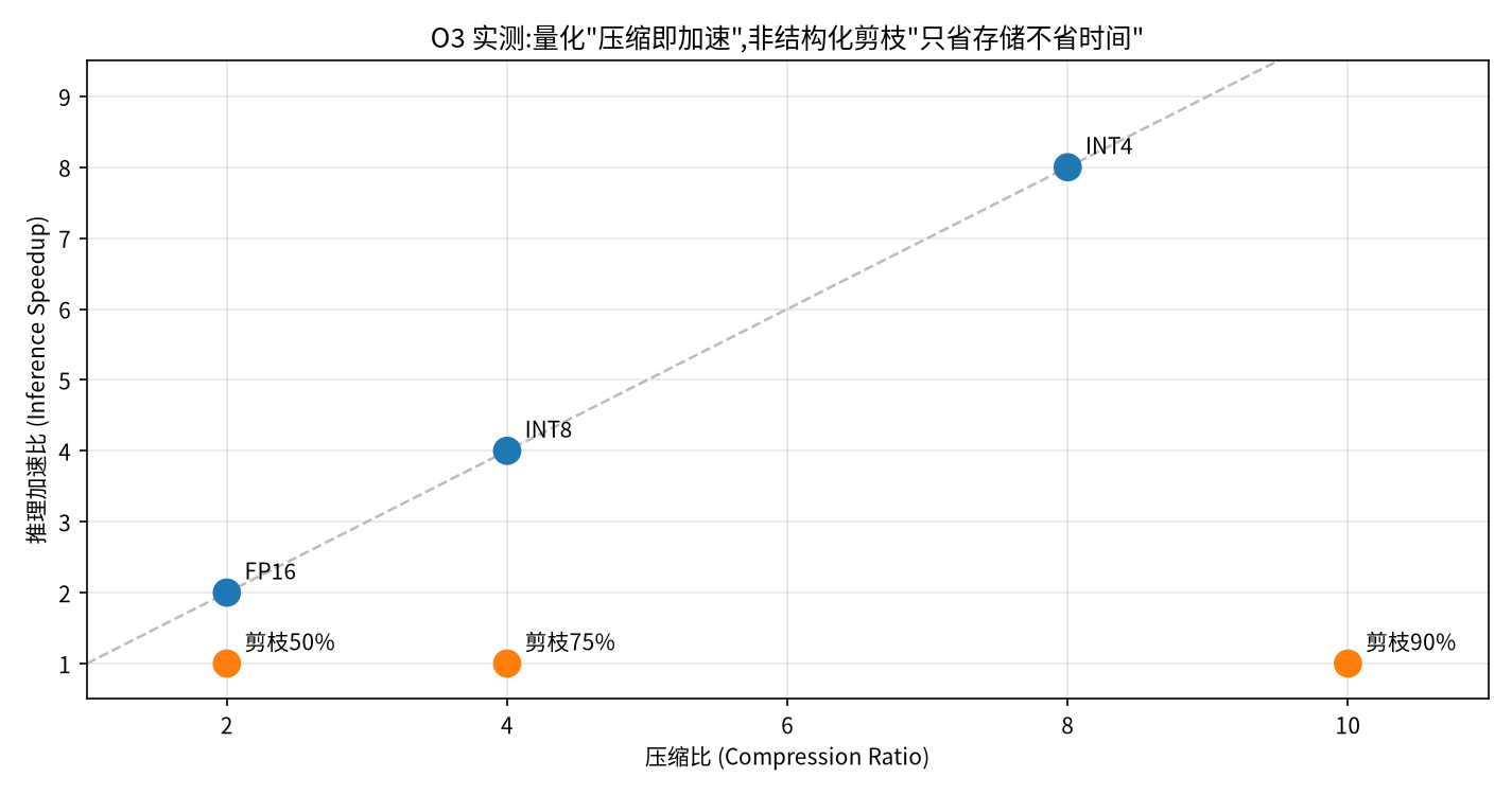
Fig 3: quantization hugs the ideal “compress 2×, speed up 2×” line; unstructured pruning speeds up exactly 1.00× no matter how much it compresses — storage saved, time unchanged.
Two patterns jump out:
- Quantization: compression ratio = speedup. INT4 compresses 8× and accelerates 8×. Quantization reduces each weight element’s bit width, so the bytes moved per Decode step shrink proportionally —
inference_speedupfaithfully mirrors “how much less data is moved”. - Unstructured pruning: huge compression, speedup stuck at 1.00×. Pruning 90% saves 90% of storage but doesn’t speed up inference by a single step. That is the most counter-intuitive and most instructive row — for unstructured pruning, saving storage and saving time are completely decoupled.
Why doesn’t unstructured pruning accelerate?
This was the core question I asked today. The answer lies in a double mismatch of hardware and sparsity pattern:
- GPUs are designed for dense GEMM. The heart of neural inference is matrix multiplication; Tensor Cores assume every matrix position holds a valid number and stream at full throughput in tiles. There is no hardware logic for “skip if the value is zero”.
- Unstructured pruning produces “random sparsity”. Zeroing the smallest-magnitude weights element-wise scatters zeros randomly across the matrix — a pattern that matches neither the dense-compute paradigm nor any hardware-recognized regular sparsity.
- “Fits in memory” and “computes fast” are two different pipelines. After pruning you can store only the non-zero values in a compressed format, so the model file gets smaller; but at compute time you either decompress back to dense (no speedup) or run sparse GEMM — random sparsity’s sparse-matrix multiply speedup is near zero, plus it pays index overhead.
- Hardware-accelerated sparsity demands regular sparsity. NVIDIA’s sparse Tensor Cores (Ampere and later) support the 2:4 pattern (exactly 2 zeros per 4 elements) at 2× speedup, but only if the pruning algorithm deliberately conforms to that pattern. Ordinary unstructured pruning (random zero distribution) doesn’t qualify.
Against Fig 3 it’s clear: quantization makes each number shorter, directly cutting bytes moved; unstructured pruning erases some numbers, cutting storage but not the per-step byte count — because sparse matrices still go through dense GEMM on ordinary hardware. This is also the fundamental reason quantization is far more common in production than unstructured pruning.
(One clarification: the engine’s estimated_accuracy_delta is a simplified static estimate — the local numbers (-0.03% ~ -0.06%) are far gentler than the “INT4 loses 2.5%” often quoted in tutorials. It shows the direction of the trade-off, not a real evaluation — see Section 6.)
5. Questions Met Along the Way
Q1: Is PagedAttention a GPU mechanism or a model mechanism?
Neither. PagedAttention is a software memory-management algorithm implemented by the inference engine (vLLM) — analogous to virtual memory/page tables in an OS: it maintains a “block table” underneath that stitches physically scattered blocks into a logically contiguous memory region to feed the model. The GPU hardware only understands contiguous physical addresses; the model only does math; the engine does the translation in between. That’s the key to the last section of the tutorial: it solves the engineering problem of memory fragmentation and redundancy, not a model-structure problem.
Q2: Why do Static / Paged-16 / Paged-64 produce identical results?
The tutorial and task both show an experiment where only page_size changes (2048 / 16 / 64) and Max Users, Throughput, Frag, Speedup come out identical. My local run reproduced it exactly (seq_len=32768, max_batch=16):
System             Max Users  Throughput  Frag  Speedup
───────────────────────────────────────────────────────
Static (baseline)         16     632 t/s  0.0%     1.1x
Paged (16 tok)            16     632 t/s  0.0%     1.1x
Paged (256 tok)           16     632 t/s  0.0%     1.1x
Three stacked reasons:
seq_lendivides evenly bypage_size, so fragmentation is naturally 0. Tutorial default seq_len=4096: ÷2048=2, ÷16=256, ÷64=64 — all exact, perfect fill,Fragall 0.0%. PagedAttention removes waste; with no waste to remove it has nothing to do.max_batch_sizecaps concurrency. All three configurations are pinned by the same ceiling (16); memory never becomes the bottleneck.- All requests live and die together. In the simulator every request has the same length and the same lifecycle; no short request finishes early to free space — “allocate on demand + reuse dynamically” has zero room to play.
I changed seq_len to 4000 and raised max_batch_size to 1000 to make memory the bottleneck, and finally saw a difference: Static fits 130, Paged-16 fits 133, Paged-64 fits 132. The difference exists, but is far smaller than intuition suggests.
Q3: When does PagedAttention actually pay off?
The key insight: PagedAttention is a “space” optimization, Continuous Batching is a “time” optimization; combined they amplify throughput to the extreme.
- PagedAttention eliminates space waste: physical blocks allocated on demand, prefix sharing (multiple requests with the same system prompt share one KV copy), copy-on-write.
- Continuous Batching eliminates time waste: whoever finishes first releases first, and the freed slot is immediately taken by a new request.
- Only when request lengths follow a long-tail distribution (80% short + 20% long) do short requests release memory quickly and PagedAttention fill the gaps dynamically — that is when the two produce a real 1+1>2. The simulator’s “requests live and die together” setup removes the time dimension, so the space optimization can’t express itself either.
This also explains why the tutorial puts PagedAttention in the “memory utilization” lesson: like quantization, it makes better use of the wall’s interior rather than pushing the wall.
Q4: INT4 speedup rises with batch instead of falling?
Optional experiment O2’s wording is “show the FP16 vs INT4 ITL comparison across batch sizes and find the critical batch size where INT4 speedup starts declining”. My prior was: as batch grows, LLM inference eventually shifts from memory-bound to compute-bound, the bytes quantization saves stop mattering, and speedup should fall.
Measured results (H100, 8B, seq 2048) say otherwise:
| Batch | ITL fp16 | ITL int4 | Speedup |
|---|---|---|---|
| 1 | 5.19 ms | 1.54 ms | 3.38× |
| 2 | 5.27 ms | 1.56 ms | 3.38× |
| 4 | 5.43 ms | 1.60 ms | 3.40× |
| 8 | 5.76 ms | 1.68 ms | 3.43× |
| 16 | 6.40 ms | 1.84 ms | 3.48× |
| 32 | 7.68 ms | 2.16 ms | 3.56× |
| 64 | 10.24 ms | 2.80 ms | 3.66× |
| 128 | 15.37 ms | 4.08 ms | 3.76× |
| 256 | 25.63 ms | 6.65 ms | 3.86× |
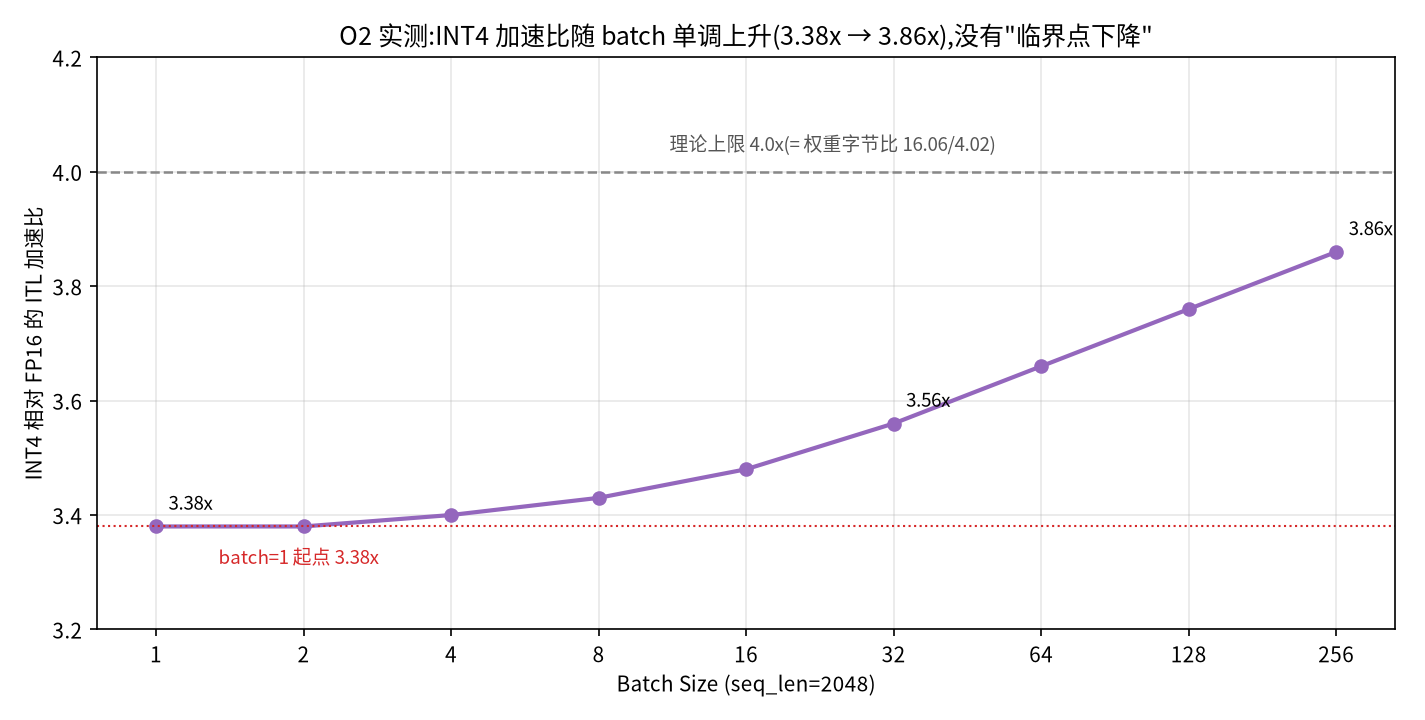
Fig 4: INT4 vs FP16 ITL speedup climbs monotonically from 3.38× at batch=1 to 3.86× at batch=256. There is no “critical point” decline.
The speedup doesn’t decay — it climbs, asymptotically approaching the theoretical limit of 4×. Two reasons:
- Why “larger batch → compute-bound” is wrong: arithmetic intensity saturates — it isn’t pinned at 1. The intuition “batch grows → FLOPs grow linearly, weights are read only once → eventually compute-bound” silently assumes the denominator contains only weights. Put KV into the denominator and it changes:
AI(B) = 2·N·B / (N·b_w + B·KV_req)
At small batch the weights dominate: AI ≈ 2B/b_w, growing linearly with B — the intuition holds in this regime. At large batch KV dominates: AI converges to 2N/KV_req and stops growing. At seq=2K that saturation value is 60 FLOP/byte (Llama-3-8B: N = 8.03B, KV_req = 0.268 GB), while the H100 ridge is 295 (989 TFLOP/s ÷ 3.35 TB/s; still ~148 at the engine’s default 0.5 efficiency) — a fivefold gap no batch can close. It’s not that the compute is too small — it’s that KV traffic grows exactly as fast as compute (both ∝ B), so the ratio converges to a constant. The ResNet-50 instinct (“crank the batch, cross the ridge”) simply doesn’t transfer to decode.
Worth untangling a pair of easily-confused questions here: AI answers “which wall do you hit” (compute vs bandwidth); speedup answers “who dominates inside the wall” (what share of the traffic is compressible). “Memory-bound forever” does not mean “speedup stays constant” — the composition of the traffic inside the wall changes with batch, which is exactly why the real-system speedup falls in Q5: not because the wall changed, but because the creditor inside it did.
- In the tool the ratio is locked at 4×. Because the engine scales KV-Cache with precision too (bytes_per_elem follows precision, so INT4’s KV is quartered, see Q5), FP16’s ledger is “16.06 GB + B·KV” and INT4’s is “4.02 GB + B·KV/4” — every term shrinks by the same factor, so the theoretical speedup is exactly 4.00×, independent of batch. Then what is the 3.38→3.86 “rise”? Fixed overhead amortizing: every generated token carries a fixed per-layer tax (32 layers × 10 μs = 0.32 ms, dug out in Part 1). At small batch the tax is ~6% of ITL, pinning speedup at 3.38; the larger the batch, the longer the memory time, the smaller the tax’s share, and the speedup monotonically approaches 4×. In the tool there is no “rising speedup” mechanism — only amortization.
So the “critical batch” the task asks about can’t be found in the tool — the tool’s assumptions hide the decline: KV scales with precision (every traffic term shrinks proportionally), and the ITL model has no compute ceiling. In real systems the critical batch does exist — driven by KV, not compute — see Q5.
Q5: Why does the engine’s INT4 KV-Cache shrink too?
A follow-up to Q4. In real deployments the KV-Cache normally stays FP16 (or gets its own dedicated KV quantization) — a separate concern from weight quantization. But mlsysim’s ServingModel binds bytes_per_elem to precision, so at INT4 the KV elements count as 0.5 bytes each — hence int4’s KV (0.070 GB @bs1) is a quarter of fp16’s (0.268 GB) in the O2 table above. That’s a simplification the engine makes, not a deployment convention. Its benefit: the “quantization speedup” experiment cleanly approaches the weight-byte ratio. Its cost: if you want to model a real system (INT4 weights + FP16 KV), you have to manually add the KV part back. Knowing which assumptions the engine made for you is something no documentation will tell you.
What about real deployments? KV normally stays FP16 (or gets its own dedicated quantization) — weight quantization can’t touch it. Restore KV to FP16 and run the same bandwidth model for “INT4 weights + FP16 KV”. The bytes moved per decode step split into two piles: weights — constant, compressible (16.06 → 4.02 GB); KV — 0.268 GB × B, incompressible. This gives the speedup a clean form — a share-weighted harmonic mean:
speedup(B) = 1 / (f_w/4 + f_kv)
where f_w is the weight share of the traffic and f_kv the KV share (f_w + f_kv = 1). Only the weight share can be divided by four; the KV share stays as is:
| Batch | Weight share f_w | KV share f_kv | Speedup |
|---|---|---|---|
| 1 | 98.4% | 1.6% | 3.81× |
| 16 | 78.9% | 21.1% | 2.45× |
| 32 | 65.2% | 34.8% | 1.96× |
| 64 | 48.4% | 51.6% | 1.57× |
| 128 | 31.9% | 68.1% | 1.31× |
| 256 | 19.0% | 81.0% | 1.17× |
Read the two sets of numbers together and the apparent contradiction dissolves: AI climbs from 1.0 to 48.6 (B=256) toward a saturation limit of 60 — still five times short of the H100 ridge at 295, so the workload stays memory-bound the whole way (memory time is always 6×+ the compute time; 25.3 ms vs 4.2 ms at B=256). Meanwhile the weight share falls from 98.4% to 19.0%, dragging speedup from 3.81× to 1.17×. One sentence: AI saturating means you never crossed the wall; speedup falling means the creditor inside the wall changed — the compressible weights get diluted to a constant, and compressing them stops paying off.
The “critical batch” the task asks you to find genuinely exists in real systems: it crosses 2× around batch≈30 at seq 2K (derived from 2B·KV = W), and earlier with longer contexts; the 50/50 crossover where KV traffic overtakes weights sits at batch≈60 (≈15 at 8K, ≈4 at 32K). The tool never shows this decline because both “drop channels” are closed: KV scales with precision (every traffic term shrinks by the same factor and cancels out, pinning speedup at exactly 4.00×), and the ITL model is pure bytes/bandwidth with no roofline ceiling — you can’t even see a compute cap.
To model the real system, add the FP16 KV back by hand — two lines on top of Script 2:
# INT4 weights, FP16 KV (the real deployment habit)
kv_fp16 = model.get_kv_cache_size(seq_len=2048, batch_size=B, precision="fp16")
total_int4 = model.size_in_bytes("int4") + kv_fp16      # not W_int4 + B*kv_int4
speedup    = (model.size_in_bytes("fp16") + kv_fp16) / total_int4
6. Two Details Dug Out of the Engine Source
Continuing the habit from Parts 1 and 2, I took CompressionModel and ServingModel apart:
Detail one: CompressionModel.solve()’s signature and result.
CompressionModel.solve(
    model, hardware,
    method="quantization",   # "quantization" | "pruning" | "distillation"
    target_bitwidth=8,       # 4, 8, 16 (quantization)
    sparsity=0.0,            # 0.0–1.0 (pruning)
    sparsity_type="unstructured"  # "unstructured" | "structured" | "n_m"
) → CompressionResult
CompressionResult fields: compressed_size_gb, compression_ratio, memory_savings_pct, inference_speedup, estimated_accuracy_delta.
Detail two: the three semantic families must be read separately. compression_ratio and memory_savings_pct are two ways of saying the same thing (ratio = 1/(1−savings)). inference_speedup equals the compression ratio under quantization but stays 1.00× under pruning — it models “the ratio of bytes moved in Decode”, not real compute change; and estimated_accuracy_delta is a lookup-table static estimate (locally -0.00% ~ -0.06%, clearly optimistic) — fine for direction, not for conclusions. Real accuracy loss needs calibration + evaluation, beyond what a simulation tool can do. The tool’s value is drawing the storage-vs-time trade-off clearly; leave “accuracy” to real evaluation.
7. Personal Takeaways
-
The memory ledger is a multiplication problem. Every factor in the KV-Cache formula (layers, KV heads, head_dim, seq_len, batch, bit width) multiplies with zero sharing or amortization. Any factor doubling doubles the memory — long context, high concurrency, and high precision cannot all fit on an 80 GB card at once. “Where did the memory go?” The answer: the multiplicands ate it.
-
Sequence length is a more insidious memory killer than model size. Weights are static (paid once at purchase); KV-Cache is dynamic (grows with every request’s context). 130 concurrent requests at 4K vs 4 at 128K — the same Llama-3-8B on the same H100 serves completely different products. Context length is a product decision that translates directly into a cost decision — which is why “128K context” is a marketing bullet point and an operations bill at the same time.
-
Quantization/pruning solves capacity — correction: quantization solves both, pruning only one. Quantization cuts bytes per element, which simultaneously cuts decode time (bandwidth wall: less to move) and total footprint (capacity wall); unstructured pruning cuts only storage, not movement. Before picking an optimization, ask which side of the wall you’re hitting: cut memory → prune; cut time → quantize (or 2:4 sparsity).
-
The simulation tool’s simplifications are its boundaries. KV scaling with precision, static accuracy_delta — both are simplifications the engine makes to teach mechanisms clearly. When using a tool for decisions, you must know which numbers are mechanism (reliable) and which are assumptions (reference only). Where the tool ends is where you go back to the real system to run the experiment. Q4/Q5 is the case in point: the same experiment shows a speedup locked at 4× in the tool and falling to 1.2× in reality — the entire gap comes from a single assumption, “KV scales with precision” — and the moment you restore FP16 KV, the task’s “critical batch” reappears.
8. References & Reproduction
- Tutorial chain: 00 Hello Roofline (Part 1) → 01 Memory Wall + 02 Two Phases (Part 2) → 03 KV-Cache: The Hidden Memory Consumer (this post) → Quantization: Not a Free Lunch (this post).
- Task: Datawhale llm-algo-leetcode #133.
- Reproduction:
pip install mlsysim, full scripts in the appendix below. - The KV-Cache formula and concurrency derivation reference the official blog: How much memory is needed for Llama 3 70B?.
- Environment: WSL2 + conda env mlsysim (python 3.11, mlsysim 0.1.1), no GPU involved — pure simulation.
Appendix: Full runnable scripts
Script 1: The KV-Cache memory ledger (E1+E2+E3) — weight sizes, KV growth vs sequence length, concurrency ceiling, and the PagedAttention comparison
import mlsysim
from mlsysim.solvers import ServingModel
from mlsysim.show import table, info

model = mlsysim.Models.Language.Llama3_8B
hardware = mlsysim.Hardware.Cloud.H100
solver = ServingModel()

# E1: weight sizes at different precisions
print("--- Llama-3-8B weights ---")
for prec, byte in [("fp16", "2 byte"), ("int8", "1 byte"), ("int4", "0.5 byte")]:
    print(f"{prec}: {model.size_in_bytes(precision=mlsysim.ureg(byte)).to('GB'):.2f} GB")
print(f"70B fp16: {mlsysim.Models.Language.Llama3_70B.size_in_bytes(precision=mlsysim.ureg('2 byte')).to('GB'):.1f} GB (H100 = {hardware.memory_capacity.to('GB'):.1f} GB)")

# E2: KV-Cache per request vs sequence length
from mlsysim.core import calc_kv_cache_size
rows = []
for ctx in [2048, 4096, 32768, 131072]:
    kv = calc_kv_cache_size(n_layers=model.layers, n_heads=model.kv_heads,
                            head_dim=model.hidden_dim // model.heads,
                            seq_len=ctx, batch_size=1, bytes_per_elem=2)
    rows.append([ctx, f"{kv.to('MB'):.0f} MB"])
table(["SeqLen", "KV per request"], rows)

# E3: concurrency ceiling sweep (feasible)
rows = []
for ctx in [2048, 4096, 32768, 131072]:
    best = 0
    for b in range(1, 1500):
        r = solver.solve(model=model, hardware=hardware, seq_len=ctx, batch_size=b, precision="fp16")
        if r.feasible:
            best = b
        else:
            break
    rows.append([ctx, best])
table(["SeqLen", "Max concurrent"], rows)

# PagedAttention comparison (why the three configs are identical:
# seq_len divides evenly by page_size + max_batch caps the ceiling)
from mlsysim.solvers import ContinuousBatchingModel
cb = ContinuousBatchingModel()
rows = []
for label, page in [("Static", 2048), ("Paged 16", 16), ("Paged 256", 256)]:
    c = cb.solve(model=model, hardware=hardware, seq_len=32768,
                 max_batch_size=16, page_size=page, precision="fp16")
    rows.append([label, c.max_active_requests, f"{c.throughput_tokens_per_sec:.0f} t/s",
                 f"{c.memory_fragmentation_pct:.1f}%", f"{c.speedup_vs_static:.1f}x"])
table(["System", "Max Users", "Throughput", "Frag", "Speedup"], rows)
Script 2: Quantization & compression (O1+O2+O3) — 8B→70B, INT4 speedup vs batch, CompressionModel quantization vs pruning
import mlsysim
from mlsysim.solvers import ServingModel, CompressionModel
from mlsysim.show import table

model = mlsysim.Models.Language.Llama3_8B
hardware = mlsysim.Hardware.Cloud.H100
solver = ServingModel()

# O1: 8B → 70B scaling of both phases
for m in [model, mlsysim.Models.Language.Llama3_70B]:
    r = solver.solve(model=m, hardware=hardware, seq_len=2048, batch_size=1, precision="fp16")
    print(f"{m.name}: TTFT {r.ttft.to('ms')}  ITL {r.itl.to('ms')}  weights {r.model_weights_size}")

# O2: INT4 speedup vs batch (conclusion: climbs monotonically, no critical point)
rows = []
for b in [1, 2, 4, 8, 16, 32, 64, 128, 256]:
    r16 = solver.solve(model=model, hardware=hardware, seq_len=2048, batch_size=b, precision="fp16")
    r4 = solver.solve(model=model, hardware=hardware, seq_len=2048, batch_size=b, precision="int4")
    rows.append([b, r16.itl.to("ms"), r4.itl.to("ms"),
                 f"{r16.itl.to('ms').magnitude / r4.itl.to('ms').magnitude:.2f}x"])
table(["Batch", "ITL fp16", "ITL int4", "Speedup"], rows)

# O3: quantization vs pruning (compression-accuracy trade-off)
cs = CompressionModel()
rows = []
for bits in [16, 8, 4]:
    c = cs.solve(model=model, hardware=hardware, method="quantization", target_bitwidth=bits)
    rows.append([f"Q-{bits}bit", c.compressed_size_gb, f"{c.compression_ratio:.1f}x",
                 f"{c.estimated_accuracy_delta:+.2f}%", f"{c.inference_speedup:.2f}x"])
for sp in [0.5, 0.75, 0.9]:
    c = cs.solve(model=model, hardware=hardware, method="pruning", sparsity=sp, sparsity_type="unstructured")
    rows.append([f"Prune {sp:.0%}", c.compressed_size_gb, f"{c.compression_ratio:.1f}x",
                 f"{c.estimated_accuracy_delta:+.2f}%", f"{c.inference_speedup:.2f}x"])
table(["Method", "Compressed", "Ratio", "Acc Delta", "Speedup"], rows)
If this note helps you, feel free to reach out.
-
Previous
KV-Cache 的显存账本:长上下文、并发与量化剪枝的取舍The KV-Cache Memory Ledger: Long Context, Concurrency, and the Quantization–Pruning Trade-off -
Next
给开源教程修了个 demoFixing a Tutorial Demo: An Open-Source PR Retrospective
If this post helped you, a coffee is always welcome ☕