The previous post, Why Does the GPU Starve, pushed the view from single-point analysis to whole-pipeline optimization. Today I enter the fifth stage of the Datawhale mlsysim learning task, which reframes the question: going from one machine to a thousand GPUs, how does the cost change? The tutorials are 06 Scaling to 1000 GPUs, 07 Geography is a Systems Variable, and 08 The $9M Question. Two surprises: in the scale sweep table, communication overhead does not grow with scale — it falls from 1336.8 ms to 319.1 ms; and the reliability conclusion crosses over much later than the tutorial claims.
1. Results first
I ran E1 (3D parallelism), E2 (scale sweep), O1 (reliability & checkpoints), E4 (site selection), and E3 (economics) with Llama-3-70B + DGX H100 + InfiniBand NDR on mlsysim 0.1.2, pure simulation. Five things worth remembering separately:
- Communication is the bottleneck everyone quotes at thousand-GPU scale. Measured, it is only 5.6%~7.4% of step time and falls rather than rises with scale — but that is not because the network gets better; the tutorial’s table mixes two different batch conventions into one column.
- The engine’s cluster MTBF is a node-level series model: one node 4285.7 h, 512 GPUs 67.0 h. The tutorial’s “512 GPUs about 97 h” is another assumption obtained by dividing MTTF by the GPU count directly.
- The tutorial’s §5 verdict is “reliability overhead dominates communication overhead”. The direction is right, but the crossover sits near 2560 GPUs, not 1024 — at 1024 GPUs reliability loss is only 0.71x communication loss.
- For the same cluster’s 30-day job the engine carries two reliability ledgers. §5 uses “write time + half an interval of rollback”;
ReliabilityResult.goodput_ratiouses “write/interval + recovery/MTBF”. At 1024 GPUs it reports one third of §5’s number. - Site selection: the same 32 GPUs, the same 30 days, Poland emits 61.1x Quebec’s carbon. On the economics side, Capex is a constant 83.4% of a 30-day TCO — short training jobs are almost entirely depreciation, not electricity.
2. E2 scale sweep: why the table runs backwards
The tutorial’s sweep parameters: TP fixed at 8 (intra-node NVLink), PP=1 (no bubbles), DP grows with node count, batch = max(64, n_gpus):
| GPUs | Nodes | Comm (ms) | Bubble (ms) | Efficiency | Step (ms) | Throughput (tok/s) | Comm share |
|---|---|---|---|---|---|---|---|
| 8 | 1 | 1336.8 | 0.0 | 92.4% | 17,665.4 | 29.0 | 7.57% |
| 32 | 4 | 393.4 | 0.0 | 93.6% | 6,132.1 | 83.5 | 6.42% |
| 64 | 8 | 236.2 | 0.0 | 94.4% | 4,209.9 | 121.6 | 5.61% |
| 128 | 16 | 280.4 | 0.0 | 93.4% | 4,254.0 | 240.7 | 6.59% |
| 256 | 32 | 302.4 | 0.0 | 92.9% | 4,276.1 | 478.9 | 7.07% |
| 512 | 64 | 313.5 | 0.0 | 92.7% | 4,287.2 | 955.4 | 7.31% |
| 1024 | 128 | 319.1 | 0.0 | 92.6% | 4,292.8 | 1,908.3 | 7.43% |
Communication drops from 1336.8 ms to 236.2 ms, then climbs back to 319.1 ms. Efficiency sits at 92%~94% throughout — near-perfect scaling. The tutorial explains this as Amdahl’s-law communication being “manageable”.
I did not accept that table directly. The first red flag was the 8→32 step: nodes quadruple, communication falls to a third. Splitting communication into its TP and DP components makes it clear:
| GPUs | batch | DP | Local batch | TP comm | DP comm | Total |
|---|---|---|---|---|---|---|
| 8 | 64 | 1 | 64.0 | 1336.8 | 0.0 | 1336.8 |
| 32 | 64 | 4 | 16.0 | 334.6 | 58.8 | 393.4 |
| 64 | 64 | 8 | 8.0 | 167.6 | 68.6 | 236.2 |
| 128 | 128 | 16 | 8.0 | 167.6 | 112.8 | 280.4 |
| 512 | 512 | 64 | 8.0 | 167.6 | 145.9 | 313.5 |
| 1024 | 1024 | 128 | 8.0 | 167.6 | 151.5 | 319.1 |
Two things happen at once:
- TP communication is strictly linear in local batch — 20.9 ms per sample, independent of node count. But
max(64, n)pushes the global batch to 64 on a single node (local 64), and the moment you cross into multiple nodes the local batch collapses to 16, then 8. TP communication therefore falls from 1336.8 ms to a floor of 167.6 ms. - DP communication depends only on the gradient volume per rank —
params / TP— independent of global batch, and only weakly monotonic in participant count (0 → 151.5 ms, then essentially flat).
So “communication” at 8 GPUs and at 1024 GPUs is not the same quantity: the first is 8 GPUs exchanging activations for 64 samples inside one node; the second is 128 nodes synchronizing gradients. Two different quantities recorded in one column is what produced the “bigger scale, less communication” impression. Re-sweeping with a fixed batch gives the normal result:
| GPUs | DP group | DP comm | TP comm | Total |
|---|---|---|---|---|
| 8 | 1 | 0.0 | 167.6 | 167.6 |
| 32 | 4 | 58.8 | 167.6 | 226.4 |
| 128 | 16 | 112.8 | 167.6 | 280.4 |
| 512 | 64 | 145.9 | 167.6 | 313.5 |
| 1024 | 128 | 151.5 | 167.6 | 319.1 |
Communication rises monotonically with scale but the ceiling is low (319 ms, 7.4%). The conclusion itself holds — the tutorial’s “communication is manageable” is defensible — but its reasoning path is not clean.
2.1 Checking the bubble formula along the way
The tutorial gives the bubble fraction as (P-1)/(M+P-1). With 8 GPUs, TP=4, PP=2, sweeping the microbatch count:
| Microbatches M | Engine bubble_fraction | Theory (P-1)/(M+P-1) |
|---|---|---|
| 1 | 0.5000 | 0.5000 |
| 2 | 0.3333 | 0.3333 |
| 4 | 0.2000 | 0.2000 |
| 8 | 0.1111 | 0.1111 |
All four points coincide; P=4 and P=8 agree too. The engine uses the textbook naive form — no 1F1B benefit, no interleaved-scheduling compression. So microbatches in this engine buy you only “improvement in the formula”, not the engineering gains of scheduling algorithms. Worth remembering when using it for parallelism decisions.
2.2 E1’s 3D parallelism
Single node 8×H100, batch=64, fp16, sweeping TP×PP:
| TP | PP | DP | Step (ms) | Bubble share | Comm (ms) | Efficiency |
|---|---|---|---|---|---|---|
| 1 | 1 | 8 | 4,522.8 | 0.0% | 549.1 | 87.9% |
| 2 | 1 | 4 | 6,165.0 | 0.0% | 426.3 | 93.1% |
| 4 | 1 | 2 | 9,920.0 | 0.0% | 651.3 | 93.4% |
| 8 | 1 | 1 | 17,665.4 | 0.0% | 1336.8 | 92.4% |
| 1 | 2 | 4 | 9,078.7 | 50.0% | 470.7 | 63.2% |
| 4 | 2 | 1 | 25,638.6 | 50.0% | 1145.6 | 63.7% |
| 2 | 4 | 1 | 29,338.8 | 75.0% | 763.6 | 55.7% |
Three patterns: turning on PP eats half or three-quarters of the step in bubbles; TP from 1 to 4 raises efficiency monotonically (memory-wall pressure drops); TP=8 falls back.
3. O1 reliability: where the Young-Daly formula should point
The tutorial’s background text says: single-GPU MTTF 50,000 h, a 512-GPU cluster about 97 h. That is MTTF / N directly. The engine’s ReliabilityModel does not implement it that way — it computes the node first, then the cluster:
node MTBF = 1 / (8/MTTF_gpu + 8/MTTF_nic + 2/MTTF_psu)
cluster MTBF = node MTBF / node count
One node with 8 GPUs + 8 NICs + 2 PSUs, using MTTFs of 50,000 / 150,000 / 100,000 h:
node MTBF = 1 / (8/50000 + 8/150000 + 2/100000) = 4285.71 h
| GPUs | Nodes | Cluster MTBF (h) | Failures / 30 d | Mean interval | Young-Daly optimal (h) | Goodput |
|---|---|---|---|---|---|---|
| 64 | 8 | 535.7 | 1.34 | 22.3 days | 4.226 | 99.59% |
| 256 | 32 | 133.9 | 5.38 | 5.6 days | 2.113 | 99.15% |
| 512 | 64 | 67.0 | 10.75 | 2.8 days | 1.494 | 98.76% |
| 1024 | 128 | 33.5 | 21.50 | 1.4 days | 1.056 | 98.17% |
| 2048 | 256 | 16.7 | 43.01 | 0.7 days | 0.747 | 97.27% |
The tutorial’s “something fails roughly every day at 512+ GPUs” is an approximation of “10.75 failures in 30 days” (one every 2.8 days). And its background figure of 97 h is 45% higher than the engine’s 67 h — because MTTF/N counts only GPUs, not NICs and PSUs, and those three component classes are in series: any one of them failing stops the whole synchronous job.
calc_young_daly_interval implements T_opt = √(2·C·M) correctly (1.494 h matches hand calculation exactly). But the C used here has a trap:
| Assumed C | Optimal interval at 512 GPUs |
|---|---|
| 60 s (ReliabilityModel’s default argument) | 1.494 h |
| 141.2 s (real write time for 70B + Adam) | 2.292 h |
The engine does not use the same C in both places: ReliabilityModel.solve(checkpoint_time_s=60) is a default parameter, while CheckpointModel computes an actual write time of 141.2 s. Tutorial §4 and §5 both use the default 60 s — but a 988.4 GB checkpoint clearly does not fit in 60 seconds. Restore the real C and the optimal interval moves from 1.49 h to 2.29 h, a factor of half.
3.1 Checkpoint size: where 14 bytes/param comes from
| Optimizer | Size | bytes/param |
|---|---|---|
| sgd | 282.4 GB | 4.00 |
| adam | 988.4 GB | 14.00 |
| rmsprop | 282.4 GB | 4.00 |
Adam = fp32 weights + fp32 first moment + fp32 second moment = 14 bytes/param; 70.6B × 14 = 988.4 GB, matching the engine. This single number drives two consequences: writing is a storage problem, not a node problem, and the interval cannot be made very large.
3.2 Write bandwidth: 141 s → 2 s
Sweeping n_writers (interval 1 h):
| n_writers | Write time | MFU penalty at 1 h | Storage bottleneck |
|---|---|---|---|
| 1 | 141.20 s | 3.92% | True |
| 8 | 17.65 s | 0.49% | False |
| 64 | 2.21 s | 0.06% | False |
| 256 | 1.98 s | 0.05% | False |
After 8 writers the curve bends; after 64 it flattens at about 2 s — there is a hardware ceiling on writes (the engine uses a 500 GB/s filesystem cap plus an effective-bandwidth factor; 4 writers already gives 35.3 s, so the ceiling starts biting around 4). “Add storage bandwidth” is therefore a real but quickly exhausted gain, not an unbounded lever.
3.3 The tutorial’s §5: two ledgers, three answers
The tutorial’s §5 algorithm: communication loss = (1 − efficiency) × 720 h; checkpoint loss = total write time over 30 days + failures × half an interval. Recomputed with C = 141.2 s:
| GPUs | Comm loss | Write | Rollback | Reliability total | Rel/comm | Total % of 720 h |
|---|---|---|---|---|---|---|
| 64 | 40.4 | 4.4 | 4.4 | 8.7 | 0.22× | 6.8% |
| 256 | 50.9 | 8.7 | 8.7 | 17.4 | 0.34× | 9.5% |
| 512 | 52.7 | 12.3 | 12.3 | 24.6 | 0.47× | 10.7% |
| 1024 | 53.5 | 17.4 | 17.4 | 34.9 | 0.65× | 12.3% |
| 2048 | 54.0 | 24.6 | 24.6 | 49.3 | 0.91× | 14.3% |
| 2560 | 54.1 | 27.6 | 27.6 | 55.1 | 1.02× | 15.2% |
| 4096 | 54.2 | 34.9 | 34.9 | 69.7 | 1.29× | 17.2% |
| 8192 | 54.4 | 49.3 | 49.3 | 98.6 | 1.81× | 21.3% |
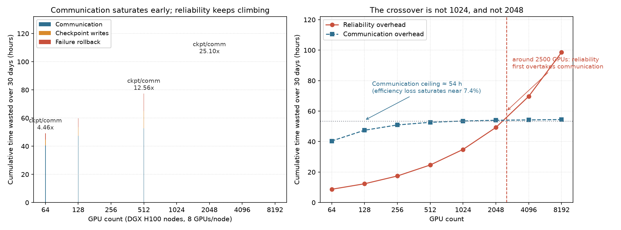
Two observations:
- Communication loss is flat, not “growing with scale”. It saturates near 7.4% (54.4 h), because the fixed terms in step latency (compute + layer tax + local TP) do not change with node count. So communication has a cap on its loss, while reliability loss rises monotonically — a crossover must exist, it just sits much later than the tutorial says.
- The crossover is near 2560 GPUs, not 1024. The tutorial’s closing claim — “at scale, reliability overhead dominates communication overhead” — is directionally right, but by its own table (0.71× at 1024 GPUs) the verb “dominates” is used a factor of two too early in scale.
The engine carries a third number internally. ReliabilityResult.goodput_ratio uses 1 − C/M − R/MTBF (C = single write time, R = recovery time 300 s). That is a steady-state share whose denominator already includes §5’s 7.4% communication loss, and whose rollback is counted as 300 s per failure rather than half an interval:
| GPUs | §5 ledger | §5 share | Goodput ledger | Goodput share | Ratio |
|---|---|---|---|---|---|
| 256 | 19.0 h | 2.65% | 6.13 h | 0.85% | 3.11× |
| 512 | 26.9 h | 3.74% | 8.93 h | 1.24% | 3.02× |
| 1024 | 38.1 h | 5.29% | 13.15 h | 1.83% | 2.90× |
| 2048 | 53.9 h | 7.48% | 19.65 h | 2.73% | 2.74× |
The three accounts differ by 3x on “how much time reliability eats”, for three different reasons: whether the denominator contains communication loss, whether rollback is half an interval or recovery time, and whether write cost is measured against ideal goodput or as a steady-state share. None is wrong, but you must state the convention when quoting — claims like “thousand-GPU training wastes 30%~50% of its time” find no support in this model: §5 gives 12.7% at 1024 GPUs, the goodput ledger gives 1.83%.
One thing worth keeping: in §5’s ledger, write and rollback are exactly equal (write = rollback in every row). That is because the Young-Daly optimum happens to split the two equally — C·(T/C) = 1 and f·(T/2) = 1 both hold at the optimal solution. So “checkpoint overhead” in this model inherently means “write plus an equal amount of rollback”, not two independent terms. The C trap from above breaks the identity in exactly the way you would expect: compute the optimal interval with the default C = 60 s but still write 141.2 s of real data, and at 64 GPUs write (6.7 h) overtakes rollback (2.8 h) — the interval is squeezed too short, so checkpoint counts rise and write dominates.
4. E4 site selection: 61x, not 40x
The E2 configuration (32 GPUs), 30 days, only the grid changes:
| Region | Energy | Carbon (t) | Total energy (MWh) | PUE | gCO₂/kWh |
|---|---|---|---|---|---|
| Norway | Hydro | 0.2 | 17.1 | 1.06 | 10 |
| Quebec | Hydro | 0.3 | 17.1 | 1.06 | 20 |
| France | Nuclear | 0.9 | 18.1 | 1.12 | 50 |
| US average | Mixed | 7.7 | 18.1 | 1.12 | 429 |
| Germany | Coal+wind | 7.0 | 18.1 | 1.12 | 385 |
| Poland | Coal | 20.9 | 25.5 | 1.58 | 820 |
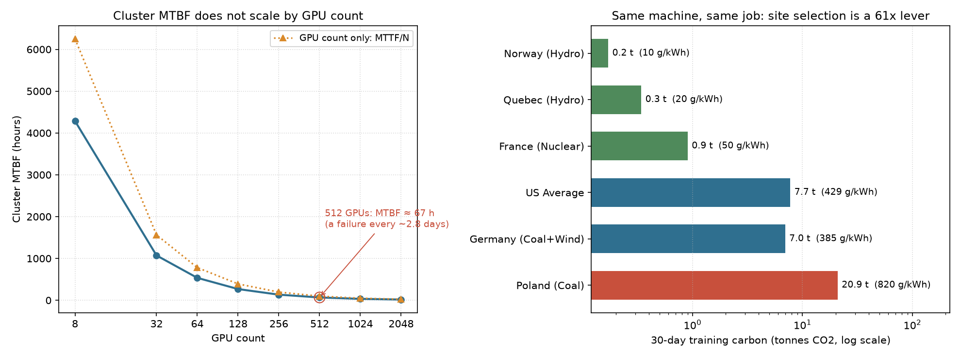
Poland/Quebec = 61.1x, Poland/US = 2.7x, Poland/Iceland = 43.7x. Tutorial 07’s repeated “40x” is the purity gap (820/20 gCO₂/kWh); the actual carbon gap also folds in PUE (1.58 vs 1.06) and energy mix (25.5 vs 17.1 MWh) — so the real number is larger than the purity gap.
4.1 Do not count operational carbon only
Sweeping embodied_carbon_per_device (Poland, 30 days):
| Embodied (kg/GPU) | Total carbon (t) | Embodied (t) | Operational share |
|---|---|---|---|
| 0 | 20.9 | 0.0 | 100.0% |
| 300 | 30.5 | 9.6 | 68.5% |
| 500 | 36.9 | 16.0 | 56.6% |
| 1000 | 52.9 | 32.0 | 39.5% |
The default is 0 — the engine counts only operational carbon. Manufacturing carbon is independent of location; it is a fixed amount amortized in. Which means “move to a hydro site” only affects operational carbon and leaves manufacturing carbon untouched; conversely, extending hardware lifetime is worth less in a low-carbon region and only pays off in a high-carbon one.
5. E3 economics: 83.4% of a 30-day bill is depreciation
The EconomicsModel conventions, confirmed in source:
Capex(period) = unit cost × GPU count × infra_multiplier / 3 years × run days / 365
maintenance  = full Capex × 5%/year × days / 365
electricity  = post-PUE energy × $0.12/kWh
H100 at $25,000 each, infra_multiplier = 2.0 (network, cooling, facility, staff):
| Days | Capex | Electricity | Maintenance | TCO | Carbon (t) | Capex share |
|---|---|---|---|---|---|---|
| 7 | $10,228 | $506 | $1,534 | $12,268 | 1.8 | 83.4% |
| 30 | $43,836 | $2,168 | $6,575 | $52,579 | 7.7 | 83.4% |
| 90 | $131,507 | $6,503 | $19,726 | $157,736 | 23.2 | 83.4% |
| 180 | $263,014 | $13,006 | $39,452 | $315,471 | 46.5 | 83.4% |
| 365 | $533,333 | $26,373 | $80,000 | $639,706 | 94.3 | 83.4% |
The Capex share is a constant 83.4%, independent of duration — because Capex, maintenance, and electricity are all prorated linearly, so their ratio is fixed. This is one form of “non-linear cost” in this model: in a short window like 30 days, almost all the money goes into a three-year depreciation, not into the electricity you actually burn.
Scale sweep (30 days, infra 2.0):
| GPUs | TCO | Capex share | Carbon (t) | Carbon per $10k TCO |
|---|---|---|---|---|
| 8 | $13,145 | 83.4% | 1.9 | 1,473.8 t |
| 32 | $52,579 | 83.4% | 7.7 | 1,473.8 t |
| 128 | $210,314 | 83.4% | 31.0 | 1,473.8 t |
| 512 | $841,257 | 83.4% | 124.0 | 1,473.8 t |
| 1024 | $1,682,514 | 83.4% | 248.0 | 1,473.8 t |
TCO scales strictly linearly with GPU count, and carbon intensity per dollar spent is constant at 1,473.8 t per $10k — in this model, scale produces no economics at all, it only multiplies the absolute amount.
infra_multiplier is the switch for “full datacenter cost”:
| mult | Capex (30 d) | Electricity | Maintenance | TCO |
|---|---|---|---|---|
| 1.0 (hardware only) | $21,918 | $2,168 | $3,288 | $27,373 |
| 2.0 | $43,836 | $2,168 | $6,575 | $52,579 |
| 2.5 | $54,795 | $2,168 | $8,219 | $65,181 |
Electricity is unchanged; Capex and maintenance double. The tutorial’s source comments say 2.0~2.5 corresponds to full facility cost and 1.0 to cards only — the default of 1.0 is an optimistic convention, and budgeting with it under-reports by roughly a factor of two.
5.1 Back to the “$9M Question”: why cost is not linear
The check-in task asks why large-scale training cost is not linear. In this model I found non-linearity in only three places, and none of them is a scale elasticity of the “bigger is cheaper/expensive” kind:
- The amortization window. Capex is spread straight-line over 3 years, so a 30-day job absorbs
30/365/3 = 2.7%of the hardware’s life. Running the same cluster for a full year, the Capex share goes from 83.4% to…… still 83.4% (because all three terms are linear). What actually changes the structure is: if the hardware runs continuously for 3 years rather than 30 days, Capex is amortized 12x more, and only then does electricity rise as a share. So the non-linearity comes from utilization, not from scale. - Reliability. Under §5’s ledger, 12.7%~22.5% of 30 days is wasted — time on already-paid-for machines. Of the $1.68M TCO for 1024 GPUs over 30 days, roughly $200k~$380k is pure waste, and that grows super-linearly with scale (1.81× at 8192).
- Site selection. Carbon intensity per dollar is constant, but carbon itself is not proportional to scale — it tracks PUE, which is a regional attribute.
One line for this section: in this engine, “scale” is not a cost lever — it is a switch on the time axis. Cost structure is set by run duration, amortization horizon, and reliability, not by GPU count. That runs against intuition, but it matches the judgement that “training a model is mainly buying time”.
6. Putting the two ledgers together: this chart is worth keeping
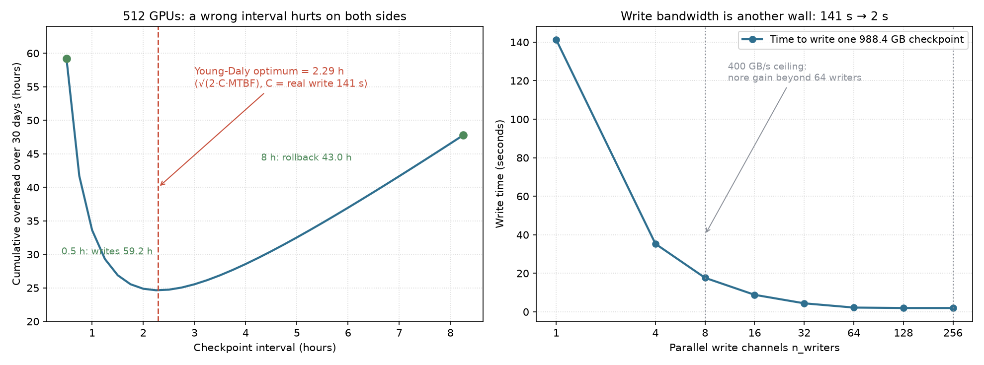
Left: the 512-GPU interval sweep. With C = 141.2 s the Young-Daly optimum is 2.29 h, 24.6 h of loss over 30 days. Picking 0.5 h writes 49.2 h; picking 8 h rolls back 43.0 h — a U shape that hurts on both ends, but flat near the optimum (2.29 h to 4 h differs by only 4.5 h). Practically: you do not need to nail the Young-Daly optimum, keeping the interval within 2x of it is close enough.
Right: the other wall — writing. The 141 s → 2 s gain comes almost entirely from 1→8 writers; past 64 the curve flattens. So “add storage bandwidth” and “tune the checkpoint interval” are different kinds of spend: the first is a one-time investment for about 1% MFU, the second is free and buys 3~7% of a 30-day loss.
7. Personal note: today’s biggest takeaway was “conventions”
This stage was not technically hard — but after running it, what I found is that the easiest thing to get wrong is not the formula, it is the convention. Four specific cases:
- Communication falling with scale. On the surface, “the network is good”; in fact
max(64, N)breaks the batch convention between 8 and 32 GPUs. Two different quantities in one column, invisible to the eye. - Is MTBF 67 h or 97 h? The tutorial’s background uses MTTF/N; the engine uses node series. A 45% difference. Both are right, but they model different failure assumptions — the first assumes only GPUs fail, the second assumes a NIC or PSU can also stall the whole job. The latter is closer to reality.
- How much time does reliability eat? §5’s ledger, the goodput ledger, and whichever C you choose combine into a range of 1.8%~12.7%. The “10-30%” quoted in the tutorial’s key-insight box runs high for this model.
My habit going forward: before quoting a tutorial’s conclusion, reproduce its conventions first. E2’s table, taken as a conclusion, is “communication manageable, reliability dominates” — fine. But once you use it to decide (“should I change the checkpoint interval from 2 h to 1 h?”), a 3x convention error flips the decision.
The positioning of this tool is now clear too: it is a calculator that writes its assumptions down, not an oracle that hands you answers. Its value is that every number it gives you can be interrogated — what is C here, does the denominator include communication loss, is this batch global or local? Those questions are, for the most part, what distributed systems design consists of.
8. References and reproduction
- Tutorial chain: 00 Hello Roofline(part 1) → 01+02 Memory Wall & Two Phases(part 2) → 03 KV-Cache(part 3) → 04 Starving the GPU + 12 DSE(part 4) → 06 Scaling to 1000 GPUs + 07 Geography + 08 The $9M Question (this post).
- Check-in task: Datawhale llm-algo-leetcode #137.
- Reproduction:
pip install mlsysim; the full script is in the appendix below, all runnable directly (pure simulation, no GPU needed). - Environment: WSL2 + conda env mlsysim (python 3.11, mlsysim 0.1.2), no GPU throughout.
Appendix: full script (copy and run)
"""
MLSysBook Task 5 - appendix reproduction script
E2 scale sweep / E1 bubble formula / O1 reliability+checkpoint / E4 geography / E3 economics
Env: pip install mlsysim (0.1.2 for this post) - pure simulation, no GPU needed
"""
import warnings
warnings.filterwarnings("ignore")
import mlsysim
from mlsysim import Models, Systems
from mlsysim.solvers import (DistributedModel, ReliabilityModel, CheckpointModel,
                             EconomicsModel, SustainabilityModel)
from mlsysim.systems.types import Fleet
from mlsysim.systems.reliability import Reliability as REL
from mlsysim.infrastructure.registry import Grids

model = Models.Language.Llama3_70B
solver, rel, ckpt = DistributedModel(), ReliabilityModel(), CheckpointModel()
econ, sust = EconomicsModel(), SustainabilityModel()
JOB = 30 * 24

def fl(n):
    """DGX H100 node (8 GPUs) + InfiniBand NDR"""
    return Fleet(name=f"{n}-GPU", node=Systems.Nodes.DGX_H100,
                 count=n // 8, fabric=Systems.Fabrics.InfiniBand_NDR)

# -- E2: scale sweep, with communication split into TP and DP components --
print("E2  Why does communication fall with scale? (TP=8 fixed, batch=max(64,N))")
print(f"{'GPUs':>6} {'batch':>6} {'DP':>4} {'localB':>7} {'TPcomm':>8} {'DPcomm':>8} {'total':>8} {'eff':>7}")
for n in [8, 32, 64, 128, 256, 512, 1024]:
    r = solver.solve(model=model, fleet=fl(n), batch_size=max(64, n),
                     precision="fp16", tp_size=8, pp_size=1)
    print(f"{n:>6} {max(64,n):>6} {r.parallelism['dp']:>4} {max(64,n)/(n//8):>7.1f} "
          f"{r.tp_communication_latency.to('ms').magnitude:>8.1f} "
          f"{r.dp_communication_latency.to('ms').magnitude:>8.1f} "
          f"{r.communication_latency.to('ms').magnitude:>8.1f} {r.scaling_efficiency:>7.1%}")

# -- E1: bubble formula check (P-1)/(M+P-1) --
print("\nE1  Bubbles: engine vs theory (P-1)/(M+P-1)   8 GPU, TP=4 PP=2")
for mb in [1, 2, 4, 8]:
    r = solver.solve(model=model, fleet=fl(8), batch_size=64, precision="fp16",
                     tp_size=4, pp_size=2, microbatch_count=mb)
    print(f"  M={mb}: engine {r.bubble_fraction:.4f}   theory {(2-1)/(mb+2-1):.4f}")

# -- O1: node-level MTBF + Young-Daly + checkpoint ledger --
print("\nO1  Node-level MTBF and Young-Daly (C=60s default)")
node_mtbf = 1 / (8/REL.Gpu.mttf_hours + 8/REL.Nic.mttf_hours + 2/REL.Psu.mttf_hours)
print(f"  single-node MTBF = {node_mtbf:.2f} h (8 GPU + 8 NIC + 2 PSU in series)")
print(f"{'GPUs':>6} {'MTBF(h)':>9} {'fail/30d':>9} {'mean intv(d)':>13} {'Young-Daly(h)':>14} {'goodput':>8}")
for n in [64, 256, 512, 1024, 2048]:
    r = rel.solve(fl(n), JOB, checkpoint_time_s=60.0)
    print(f"{n:>6} {r.fleet_mtbf.to('hour').magnitude:>9.1f} {r.expected_failures:>9.2f} "
          f"{JOB/r.expected_failures/24:>13.2f} "
          f"{r.optimal_checkpoint_interval.to('hour').magnitude:>14.3f} {r.goodput_ratio:>8.2%}")

print("\nO1  Checkpoint size (bytes/param) and write bandwidth")
for opt in ["sgd", "adam"]:
    r = ckpt.solve(model=model, hardware=Systems.Nodes.DGX_H100.accelerator,
                   optimizer=opt, checkpoint_interval_hours=1.0)
    print(f"  {opt:<5}: {r.checkpoint_size.to('GB').magnitude:>7.1f} GB  "
          f"= {r.checkpoint_size.to('B').magnitude/model.parameters:.2f} bytes/param")
for w in [1, 8, 64, 256]:
    r = ckpt.solve(model=model, hardware=Systems.Nodes.DGX_H100.accelerator, optimizer="adam",
                   checkpoint_interval_hours=1.0, n_writers=w)
    print(f"  n_writers={w:>3}: {r.write_time_seconds.to('s').magnitude:>7.2f} s  "
          f"storage_bottleneck={r.storage_bottleneck}")

print("\nO1  Two ledgers: Sec5 (write + half-interval rollback) vs engine goodput")
for n in [256, 512, 1024, 2048]:
    d = solver.solve(model=model, fleet=fl(n), batch_size=max(64, n), precision="fp16",
                     tp_size=8, pp_size=1)
    rr = rel.solve(fl(n), JOB, checkpoint_time_s=60.0)
    ci = rr.optimal_checkpoint_interval.to("hour").magnitude
    w_s = ckpt.solve(model=model, hardware=Systems.Nodes.DGX_H100.accelerator, optimizer="adam",
                     checkpoint_interval_hours=ci).write_time_seconds.to("s").magnitude
    sec5 = JOB/ci*w_s/3600 + rr.expected_failures*(ci/2)
    gp = (1 - rr.goodput_ratio) * JOB
    print(f"  {n:>5} GPU: Sec5={sec5:>6.1f}h ({sec5/JOB:>5.2%})  goodput={gp:>5.2f}h ({1-rr.goodput_ratio:>5.2%})"
          f"  ratio {sec5/gp:.2f}x  comm_loss={(1-d.scaling_efficiency)*JOB:>5.1f}h")

# -- E4: geography --
print("\nE4  Same 32xH100, 30 days, only the grid changes")
for g in [Grids.Norway, Grids.Quebec, Grids.France, Grids.US_Avg, Grids.Germany, Grids.Poland]:
    r = sust.solve(fleet=fl(32), duration_days=30, datacenter=g)
    print(f"  {r.region_name:<22} {r.carbon_footprint_kg/1000:>6.1f} t  "
          f"PUE {r.pue:.2f}  {g.carbon_intensity_g_kwh:>5.0f} g/kWh")

# -- E3: economics --
print("\nE3  TCO: scale sweep (30 days, infra 2.0)")
print(f"{'GPUs':>6} {'TCO':>13} {'CapexShare':>11} {'Carbon(t)':>10} {'t per $10k TCO':>17}")
for n in [8, 32, 128, 512, 1024]:
    r = econ.solve(fleet=fl(n), duration_days=30, infrastructure_multiplier=2.0)
    print(f"{n:>6} {r.tco_usd:>13,.0f} {r.capex_usd/r.tco_usd:>11.1%} "
          f"{r.carbon_footprint_kg/1000:>10.1f} {r.carbon_footprint_kg/(r.tco_usd/1e4):>17.1f} t")
If this note was useful, I’d be glad to talk.
-
Previous
给开源教程修了个 demoFixing a Tutorial Demo: An Open-Source PR Retrospective -
Next
千卡训练的隐形账单:通信不是瓶颈The Hidden Bill of Thousand-GPU Training: Communication Is Not the Bottleneck
If this post helped you, a coffee is always welcome ☕