In The KV-Cache Memory Ledger, I flipped the lens from “time” to “space” and accounted for where the memory goes. Today I moved on to the fourth stage of the Datawhale mlsysim study activity, widening the view from single-point performance analysis (Tasks 1-3) to systematic optimization. This maps to three tutorials: 04 Starving the GPU, 12 Design Space Exploration, and the optional Module 2: Advanced Single-Node Analysis. The core question is blunt: when GPU utilization sits at 40%, the problem usually is not the GPU — so where is the bottleneck hiding?
1. From Single-Point Bottlenecks to a Whole-Pipeline View
The first three posts were all single-point analyses: roofline tells us whether a workload is compute- or memory-bound, the memory wall quantifies how much faster a hardware upgrade really is, and the KV-Cache ledger accounts for memory. But in a real system, a training step is never the GPU working alone — it is a pipeline:
storage I/O (move samples from disk to RAM) -> CPU preprocessing (decode, augment) -> GPU compute
The three stages run in series, so end-to-end throughput is set by the slowest one:
t_step = max(t_io, t_cpu, t_gpu)      # step time is set by the slowest stage
U      = t_gpu / t_step               # GPU utilization
That is the core intuition of the Data Wall: no matter how fast the GPU is, if the stages feeding it cannot keep up, the end-to-end throughput does not move. This stage uses three mlsysim models to check the pipeline segment by segment.
2. E1: Find the GPU “Ceiling” First
First, establish the baseline: how fast is the pure GPU compute of ResNet-50 on an A100, batch=256, FP16? This becomes the baseline every other stage is compared against.
model = mlsysim.Models.Vision.ResNet50
hardware = mlsysim.Hardware.Cloud.A100
solver = SingleNodeModel()
profile = solver.solve(model=model, hardware=hardware, batch_size=256, precision="fp16")
Measured result:
| Metric | Value |
|---|---|
| Step latency | 13.97 ms |
| Throughput (ceiling) | 18,323 img/s |
| Bottleneck | Compute |
The GPU can “eat” 18,000 images per second. Keep this number — it is the ruler for every comparison that follows.
3. E2: Can Storage I/O Keep Up?
The data the GPU needs must first move from storage into memory. Say each image is a 500KB JPEG (the ImageNet average); at batch=256 one step needs 256 x 500KB = 128MB, and the GPU wants a fresh batch every 13.97 ms. Convert that to a bandwidth requirement:
demand = 256 x 500KB / 13.97 ms ~ 9.16 GB/s
DGX A100 storage rides PCIe Gen4 x16, 32 GB/s theoretical. Check with DataModel:
| Metric | Value |
|---|---|
| Workload demand | 9.16 GB/s |
| Storage supply (PCIe Gen4 x16) | 32.00 GB/s |
| Bus utilization | 28.6% |
| Stalled? | False |
Storage I/O is not the bottleneck — supply has more than 3x headroom. First segment green.
4. E3: CPU Preprocessing — the Real Reason the GPU Starves
The first two segments are fine, so the bottleneck must be the CPU. Say 8 workers at 250 MB/s each — 2 GB/s of preprocessing throughput total. Compare the CPU transform time against the GPU step time with TransformationModel:
| Metric | Value |
|---|---|
| CPU transform time | 64.0 ms |
| GPU step time | 13.97 ms |
| CPU is bottleneck | True |
| GPU utilization | 21.8% |
| Slowdown factor | 4.58x |
The GPU needs only 14 ms to do its work, but the CPU needs 64 ms to prepare the next batch — the GPU idles 78% of the time. That is the GPU starving: the GPU can process tens of thousands of samples per step, but 8 CPU workers can barely prepare a fraction of that.
4.1 Bigger Batches Starve It Harder
Sweep batch from 16 to 1024 (CPU throughput fixed at 2 GB/s — larger samples only widen the gap):
| Batch | GPU Step | CPU Xform | Binding | GPU Util |
|---|---|---|---|---|
| 16 | 1.36 ms | 4.00 ms | CPU | 33.9% |
| 32 | 2.20 ms | 8.00 ms | CPU | 27.5% |
| 64 | 3.88 ms | 16.00 ms | CPU | 24.2% |
| 128 | 7.24 ms | 32.00 ms | CPU | 22.6% |
| 256 | 13.97 ms | 64.00 ms | CPU | 21.8% |
| 512 | 27.43 ms | 128.00 ms | CPU | 21.4% |
| 1024 | 54.34 ms | 256.00 ms | CPU | 21.2% |
4.2 Add Workers, Find the Crossover
How many workers does it take to feed the GPU? Sweep the worker count (batch=512):
| Workers | CPU throughput | GPU utilization |
|---|---|---|
| 8 | 2 GB/s | 21.4% |
| 16 | 4 GB/s | 42.9% |
| 32 | 8 GB/s | 85.7% |
| 64 | 16 GB/s | 100.0% |
| 128 | 32 GB/s | 100.0% |
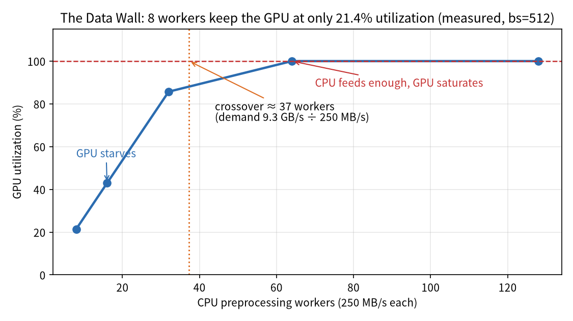
GPU utilization is almost exactly proportional to the worker count, until it hits the 100% ceiling. The crossover is computable: at batch=512 the demand is 512 x 500KB / 27.43 ms ~ 9.3 GB/s; at 250 MB/s per worker:
N_workers >= 9.3 GB/s / 250 MB/s ~ 37 workers
So roughly 37 workers is where the CPU just stops dragging its feet. That is the value of the “data wall” concept: when GPU utilization is low, inspect the supply side first — don’t blame the GPU.
The standard engineering fixes: add workers, offload preprocessing to the GPU with NVIDIA DALI, pre-decode the dataset, aggressive prefetching. The idea is always the same — keep the CPU one step ahead of the GPU.
5. E4/O1: Speculative Decoding — Let an 8B “Draft” for a 70B
There are algorithmic ways to win big with small models too. Autoregressive decoding is serial: one token at a time, and every step reads the whole model’s weights from HBM (decode is memory-bound — see Part 2). Speculative decoding flips that: a small draft model proposes K tokens, then the target model verifies them in one parallel forward pass and accepts what matches.
Expected output per round:
E(alpha) = 1 + alpha(1-alpha^K)/(1-alpha)   # expected accepted tokens
speedup  = E(alpha) / (1 + K*r)             # r = draft per-token time / target per-token time
The key: the target verifying K draft tokens is one parallel forward pass, not K serial decode steps; the draft may not guess many tokens at once, but it is cheap. So one expensive 70B stream read gets amortized over several accepted tokens.
5.1 E4: Llama-3-70B with an 8B Draft
Measured with ServingModel (H100, seq_len=2048, batch=1, alpha=0.75):
| Config | ITL | Speedup |
|---|---|---|
| Baseline (no spec decoding) | 43.15 ms | 1.00x |
| 8B draft, alpha=0.75 | 20.53 ms | 2.10x |
E(0.75)=3.05: each round drafts 4 tokens and accepts 3.05 on average. The verification step is fundamentally one 70B HBM stream read (memory-bound), and the 8B draft proposal is cheap — amortize one stream read over ~3 accepted tokens and the 2.1x comes almost for free.
5.2 O1a: Sweeping the Acceptance Rate from 0.5 to 0.9
| alpha | E(alpha) | Speedup |
|---|---|---|
| 0.50 | 1.94 | 1.33x |
| 0.75 | 3.05 | 2.10x |
| 0.90 | 4.10 | 2.82x |
The higher the acceptance rate, the steeper the gain — the better the draft guesses, the more stream-read cost each round amortizes.
5.3 O1b: How Big Should the Draft Be? Measurement Overturns a Common Intuition
Run drafts of different sizes (alpha fixed at 0.75):
| Draft model | Params | Speedup |
|---|---|---|
| GPT-2 | 1.5B | 2.77x |
| Llama-3-8B | 8B | 2.10x |
| Llama-3-70B | 70B (=target) | 0.62x |
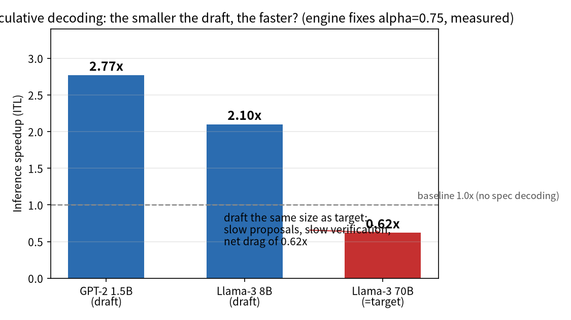
There is a gap between this and the usual story (“a draft too small -> low acceptance, too large -> exploding overhead, 8B is the compromise”): in the mlsysim engine, the acceptance rate alpha is a parameter you pass in directly — it does not automatically vary with the draft model’s size. With alpha fixed at 0.75, a smaller draft has only upsides: r shrinks, the denominator shrinks, speedup climbs — so GPT-2 wins; the 70B draft is as slow as the target itself, so proposals are slow and verification is slow, a pure overhead of 0.62x (slower than not using spec decoding at all).
The “8B” argument actually depends on something the engine does not model: in reality, alpha is a function of how close the draft’s distribution is to the target’s — a draft too small guesses poorly (low alpha), a draft too large is slow on its own (high r). By decoupling alpha from model size, the engine lets you study either effect in isolation, then combine them yourself. The real-world trade-off is “guesses well enough” vs “runs fast enough”, and the engine helps you understand the two forces separately before composing them.
6. E5: Design Space Exploration — Declarative Search Instead of Nested Loops
The third ruler is system-level. Given a cluster, which config wins on throughput across batch_size, tensor_parallelism, pipeline_parallelism, and friends? Hand-written nested for-loops work, but they get messy once dimensions multiply. mlsysim’s DSE engine takes a declarative search space and exhaustively evaluates every combination.
This run: Llama-3-70B, FP16, Frontier_8K cluster, space batch_size in [1024, 2048, 4096, 8192] x TP in [1, 2, 4, 8] x PP in [1, 2, 4] — 48 configs total, objective: maximize effective throughput:
| Rank | TP | PP | Batch | Throughput | Step latency |
|---|---|---|---|---|---|
| 1 | 8 | 4 | 8192 | 15,381 tok/s | 17,043 ms |
| 2 | 8 | 1 | 8192 | 15,245 tok/s | 4,299 ms |
| 3 | 8 | 2 | 8192 | 14,405 tok/s | 9,099 ms |
Three observations:
- TP=8 and batch=8192 sweep the podium — the search lands on the boundary of the space. On this 8K-GPU cluster, larger TP means each card holds a smaller slice of the weights (less memory pressure), while intra-node NVLink is fast enough that AllReduce cost amortizes; larger batch means the weight read is spread over more samples. Both dimensions help monotonically, so the optimum sits in a corner, not inside the space.
- PP is the latency tax: at the same TP8 x batch8192, going from PP=1 to PP=2 doubles step latency (4.3s -> 9.1s); PP=4 reaches 17s. The pipeline bubble is diluted at large batch, but the throughput gain (15,245 -> 15,381, only 0.9%) is dwarfed by the latency cost.
- A detail the engine exposes on its own: the search keeps warning
batch_size (1024) < dp_size (8192): some ranks will be idle. Frontier_8K has 8192 GPUs, and the data-parallel rank count is decided by cluster size — even batch=8192 only gives each rank 1 sample (local_batch=1). In other words, the cluster’s parallelism (8K ranks) has squeezed out the per-card batch dimension. The throughput numbers look great, but that is the credit of 8192 cards; at cluster scale, it is communication and parallelism that cap throughput, not single-card compute.
Designing the search space matters as much as the search itself: the same problem with a different space (batch from 1 to 64) gives a completely different answer — the optimum only ever lives inside the range you draw.
7. O3: Inference-Time Compute — o1 Moves the Compute Demand Back to Inference
The last topic comes from Module 2’s “Reasoning Wall”. Models like o1 run K hidden reasoning steps (chain-of-thought) before answering, and Inference-Time Compute shifts the compute demand from training back to inference. Simulate Llama-3-8B on H100 with InferenceScalingModel:
| K (hidden reasoning steps) | Total latency | Energy/query | TTFT share |
|---|---|---|---|
| 0 (no reasoning chain) | 0.071 s | 0.050 kJ | 100% |
| 8 | 2.15 s | 1.50 kJ | 3.3% |
| 32 | 8.38 s | 5.87 kJ | 0.8% |
Two key observations:
- TTFT does not move at all — prefill only processes the prompt itself; hidden reasoning happens in the decode phase. So at K=32 the TTFT share drops from 100% to 0.8%, and latency is almost entirely generation.
- Total latency and energy scale linearly with K: at K=32 one answer costs 8.38 seconds and 5.87 kJ. The systems impact is disruptive — the same GPU cluster can only serve 1/K of the concurrency. “Inference-time compute scaling” buys quality on the business side; on the systems side it is the most expensive optimization there is.
7.1 Memory Wall or Compute Wall? Where I Disagree with the Tutorial
The Module 2 summary page makes a claim: “Inference shifts back toward being compute-bound as generation length dominates prefill” — inference-time compute supposedly moves the bottleneck from the memory wall “back” to the compute wall. There are two layers to that sentence; I agree with the first and disagree with the second.
The first layer is right: compute demand really does shift from training to inference. o1 turns FLOPs that used to be spent on training into extra tokens generated at inference time. That is the essence of inference-time compute scaling, and it is the biggest systems impact — capacity planning goes from “how big should the training cluster be” to “how many FLOPs will inference burn”.
The second layer I push back on: “with generation length dominating, inference becomes compute-bound” — I think it is still stuck on the decode memory wall. Three reasons:
- Hidden reasoning tokens are just ordinary autoregressive decode. K reasoning steps are not “more compute” — they are “more decode steps”: each one streams the weights from HBM once and emits a token, structurally identical to generating a normal answer. Decode is memory-bound — measured in Part 2 (ITL is priced by HBM bandwidth). K steps of reasoning just walk that memory-bound road longer; the physics of each step does not change.
- The measurements support the memory wall, not the compute wall. If the bottleneck really flipped to compute, we should see prefill-like regime behavior; but the measurements show (a) the only compute-bound segment — prefill (TTFT) — did not move at all; (b) total latency scales strictly linearly with K, a constant per-step cost, which is exactly what “every token priced by an HBM stream read” looks like — not what a compute-bound regime looks like.
- When would the author’s claim hold? Under large-batch serving. Decode’s arithmetic intensity rises with batch (see the roofline analysis in Part 2): at high enough concurrency the GPU’s compute gets saturated and decode genuinely shifts from memory-bound to compute-bound. But that is a system-throughput shift; for a single request at low concurrency, inference-time compute is just “longer decode”, still memory-bound. This is the other side of the same coin as Part 3’s KV-Cache conclusion: long sequences are priced by memory, not by compute.
8. My Take: Three Rulers and “Find the Bottleneck First”
Task 4 condenses the single-point skills from the first three posts into a methodology. I read it as three rulers:
- Supply side (the Data Wall): when throughput stalls, look at the narrowest stage of the pipeline first; low GPU utilization is not the GPU’s fault;
- Algorithm side (speculative decoding): you can go faster without new hardware — small model proposes, target verifies, serial decoding becomes parallel verification;
- Search side (DSE): when the config space gets too big to reason about by hand, let a declarative search find the optimum.
The most valuable part is not any single formula but the “find the bottleneck, then optimize” ordering. The 4.58x slowdown in E3, the 2.10x speedup in E4, and the boundary solution in E5 all came from locating the constraint first. Optimizing blindly without knowing the bottleneck wastes effort on stages that were never the problem — like adding NVMe to storage while the real constraint sits in CPU preprocessing.
A second takeaway from Section 5.3: the draft-size result disagrees with common intuition not because anyone is wrong, but because the modeling granularity differs. The engine treats alpha as an independent knob; in reality alpha depends on draft quality. Reading the engine source and seeing what it decouples predicts “what changes if I change the conditions” better than memorizing conclusions.
9. References & Reproduction
- Tutorial chain: 00 Hello Roofline (Part 1) -> 01 Memory Wall + 02 Two Phases (Part 2) -> 03 KV-Cache (Part 3) -> 04 Starving the GPU + 12 Design Space Exploration + Module 2 (this post).
- Check-in task: Datawhale llm-algo-leetcode #136.
- Reproduction:
pip install mlsysim; the three scripts in the appendix all run directly (E1-E3 and E4/O1/O3 need no cluster; E5 uses the built-inFrontier_8Kcluster frommlsysim.Systems.Clusters). - Environment: WSL2 + conda env mlsysim (Python 3.11, mlsysim 0.1.1), no GPU involved — pure simulation.
Appendix: Full Run Scripts (Copy & Run)
Script 1: E1-E3 Data-Pipeline Analysis
import mlsysim
from mlsysim.solvers import SingleNodeModel, DataModel
from mlsysim.solvers import TransformationModel

from mlsysim.solvers import SingleNodeModel
from mlsysim.core.units import Q_
from mlsysim.show import table, info

model = mlsysim.Models.Vision.ResNet50
hardware = mlsysim.Hardware.Cloud.A100
solver = SingleNodeModel()

# Baseline: ResNet-50 on A100, batch 256, FP16
profile = solver.solve(model=model, hardware=hardware, batch_size=256, precision="fp16")

info("GPU Compute Baseline",
     Model=model.name,
     Hardware=hardware.name,
     Batch_size=256,
     Step_latency=profile.latency.to('ms'),
     Throughput=f"{profile.throughput:.0f} img/s",
     Bottleneck=profile.bottleneck)

from mlsysim.solvers import DataModel

sample_size = Q_("500 KB")  # Average ImageNet JPEG
batch_size = 256

# Data demand = batch_size x sample_size / step_time
step_time_s = profile.latency.to("s").magnitude
data_per_step = (batch_size * sample_size.to("GB")).magnitude
demand_rate = Q_(data_per_step / step_time_s, "GB/s")

data_solver = DataModel()
data_result = data_solver.solve(workload_data_rate=demand_rate, hardware=hardware)

info("Storage I/O Check",
     Data_demand=f"{demand_rate:.3f}",
     Storage_supply=f"{data_result.supply_bw:.2f}",
     Utilization=f"{data_result.utilization:.1%}",
     Is_stalled=data_result.is_stalled)

from mlsysim.solvers import TransformationModel

transform_solver = TransformationModel()
cpu_throughput = Q_("2 GB/s")  # 8 workers x 250 MB/s each

t = transform_solver.solve(
    batch_size=256,
    sample_size_bytes=sample_size,
    cpu_throughput=cpu_throughput,
    accelerator_step_time=profile.latency
)

info("CPU vs GPU Pipeline",
     CPU_transform_time=t.transform_time,
     GPU_step_time=t.accelerator_step_time,
     CPU_is_bottleneck=t.is_bottleneck,
     GPU_utilization=f"{t.accelerator_utilization:.1%}",
     Slowdown_factor=f"{t.slowdown_factor:.2f}x")

rows = []
for bs in [16, 32, 64, 128, 256, 512, 1024]:
    p = solver.solve(model=model, hardware=hardware, batch_size=bs, precision="fp16")

    t = transform_solver.solve(
        batch_size=bs,
        sample_size_bytes=sample_size,
        cpu_throughput=cpu_throughput,
        accelerator_step_time=p.latency
    )

    binding = "Transformation" if t.is_bottleneck else p.bottleneck
    rows.append([
        bs,
        f"{p.latency.to('ms').magnitude:.2f} ms",
        f"{t.transform_time.to('ms').magnitude:.2f} ms",
        binding,
        f"{t.accelerator_utilization:.1%}"
    ])

table(["Batch", "GPU Step", "CPU Xform", "Binding", "GPU Util"], rows)

rows = []
for n_workers in [8, 16, 32,64, 128]:
    cpu_tp = Q_(f"{n_workers * 250} MB/s")

    p = solver.solve(model=model, hardware=hardware, batch_size=512, precision="fp16")

    t = transform_solver.solve(
        batch_size=512,
        sample_size_bytes=sample_size,
        cpu_throughput=cpu_tp,
        accelerator_step_time=p.latency
    )

    rows.append([n_workers, cpu_tp.to('GB/s'), f"{t.accelerator_utilization:.1%}"])

table(["Workers", "Throughput", "GPU Util @ bs=512"], rows)
Script 2: E5 Design Space Exploration
import mlsysim
from mlsysim.engine.dse import DSE
from mlsysim.solvers import DistributedModel, EconomicsModel
from mlsysim.engine.pipeline import Pipeline

# Our fixed baseline constants
model = mlsysim.Models.Language.Llama3_70B
fleet = mlsysim.Systems.Clusters.Frontier_8K

# The evaluation function accepts a dictionary of parameters and returns a structured object
def evaluate_config(params):
    pipe = Pipeline([DistributedModel(), EconomicsModel()])

    return pipe.run(
        model=model,
        fleet=fleet,
        batch_size=params["batch_size"],
        tp_size=params["tp"],
        pp_size=params["pp"],
        precision="fp16",
        efficiency=0.45,
        duration_days=30
    )

# 1. Define the dimensions of your search grid
space = {
    "batch_size": [1024, 2048, 4096, 8192],
    "tp": [1, 2, 4, 8],
    "pp": [1, 2, 4]
}

# 2. Initialize the Design Space Explorer
dse = DSE(
    space=space,
    objective="maximize: DistributedModel.effective_throughput"
)

# 3. Search! (Tests all 4 * 4 * 3 = 48 combinations analytically)
print("Starting search...")

result = dse.search(evaluate_config)

# 4. Analyze the best configuration
best_params = result["best_params"]
best_throughput = result["best_objective"]

print(f"\nBest Configuration: TP={best_params['tp']}, PP={best_params['pp']}, Batch={best_params['batch_size']}")
print(f"Max Throughput: {best_throughput:,.0f} tokens/sec")

print(f"\nTop 3 Configurations:")
print(f"{'TP':>4} | {'PP':>4} | {'Batch':>6} | {'Throughput':>12} | {'Latency':>10}")
print("-" * 45)

for candidate in result["top_candidates"][:3]:
    p = candidate["params"]
    dist_res = candidate["result"]["DistributedModel"]

    throughput = dist_res.effective_throughput.m_as("1/s")
    latency = dist_res.step_latency_total.m_as("ms")

    print(f"{p['tp']:>4} | {p['pp']:>4} | {p['batch_size']:>6} | {throughput:>12,.0f} | {latency:>10.1f}ms")
Script 3: E4/O1 Speculative Decoding + O3 Inference-Time Compute
import mlsysim
from mlsysim.solvers import ServingModel, InferenceScalingModel

hw = mlsysim.Hardware.Cloud.H100
target = mlsysim.Models.Language.Llama3_70B
draft8b = mlsysim.Models.Language.Llama3_8B
draft_gpt2 = mlsysim.Models.Language.GPT2
solver = ServingModel()

# E4: baseline vs speculative decoding (8B draft, alpha=0.75)
base = solver.solve(target, hw, seq_len=2048, batch_size=1)
spec = solver.solve(target, hw, seq_len=2048, batch_size=1,
                    draft_model=draft8b, draft_acceptance_rate=0.75)
print(f"baseline ITL: {base.itl.to('ms').magnitude:.2f} ms")
print(f"spec ITL:     {spec.itl.to('ms').magnitude:.2f} ms")
print(f"speedup:      {base.itl/spec.itl:.2f}x")

# O1a: acceptance-rate sweep
for a in [0.5, 0.75, 0.9]:
    r = solver.solve(target, hw, seq_len=2048, batch_size=1,
                     draft_model=draft8b, draft_acceptance_rate=a)
    print(f"alpha={a}: ITL {r.itl.to('ms').magnitude:7.2f} ms  speedup {base.itl/r.itl:.2f}x")

# O1b: draft-model size sweep
for name, dm in [("GPT2(1.5B)", draft_gpt2), ("Llama3-8B", draft8b), ("Llama3-70B", target)]:
    r = solver.solve(target, hw, seq_len=2048, batch_size=1,
                     draft_model=dm, draft_acceptance_rate=0.75)
    print(f"draft={name}: ITL {r.itl.to('ms').magnitude:7.2f} ms  speedup {base.itl/r.itl:.2f}x")

# O3: inference-time compute (K=0/8/32)
isolver = InferenceScalingModel()
for k in [0, 8, 32]:
    r = isolver.solve(mlsysim.Models.Language.Llama3_8B, hw, reasoning_steps=k)
    print(f"K={k}: total {r.total_reasoning_time.to('s').magnitude:.3f} s  "
          f"energy {r.energy_per_query.to('kJ').magnitude:.3f} kJ")
If this note helps you, feel free to reach out.
-
Previous
GPU 为什么会挨饿:数据墙、投机解码与设计空间探索Why Does the GPU Starve: The Data Wall, Speculative Decoding, and Design-Space Exploration -
Next
给开源教程修了个 demoFixing a Tutorial Demo: An Open-Source PR Retrospective
If this post helped you, a coffee is always welcome ☕